As a kid I loved magnets. I wanted to know where the push and pull came from. Years later, when I heard about the Ising model of ferromagnetism, I became an instant fan. Here was a simple set of rules, like a game played on graph paper, that offered a glimpse of what goes on inside a magnetic material. Lots of tiny magnetic fields spontaneously line up to make one big field, like a school of fish all swimming in the same direction. I was even more enthusiastic when I learned about the Monte Carlo method, a jauntily named collection of mathematical and computational tricks that can be used to simulate an Ising system on a computer. With a dozen lines of code I could put the model in motion and explore its behavior for myself.
Over the years I’ve had several opportunities to play with Ising models and Monte Carlo methods, and I thought I had a pretty good grasp of the basic principles. But, you know, the more you know, the more you know you don’t know.
In 2019 I wrote a brief article on Glauber dynamics, a technique for analyzing the Ising model introduced by Roy J. Glauber, a Harvard physicist. In my article I presented an Ising simulation written in JavaScript, and I explained the algorithm behind it. Then, this past March, I learned that I had made a serious blunder. The program I’d offered as an illustration of Glauber dynamics actually implemented a different procedure, known as the Metropolis algorithm. Oops. (The mistake was brought to my attention by a comment signed “L. Y.,” with no other identifying information. Whoever you are, L. Y., thank you!)
A few days after L. Y.’s comment appeared, I tracked down the source of my error: I had reused some old code and neglected to modify it for its new setting. I corrected the program—only one line needed changing—and I was about to publish an update when I paused for thought. Maybe I could dismiss my goof as mere carelessness, but I realized there were other aspects of the Ising model and the Monte Carlo method where my understanding was vague or superficial. For example, I was not entirely sure where to draw the line between the Glauber and Metropolis procedures. (I’m even less sure now.) I didn’t know which features of the two algorithms are most essential to their nature, or how those features affect the outcome of a simulation. I had homework to do.
Since then, Monte Carlo Ising models have consumed most of my waking hours (and some of the sleeping ones). Sifting through the literature, I’ve found sources I never looked at before, and I’ve reread some familiar works with new understanding and appreciation. I’ve written a bunch of computer programs to clarify just which details matter most. I’ve dug into the early history of the field, trying to figure out what the inventors of these techniques had in mind when they made their design choices. Three months later, there are still soft spots in my knowledge, but it’s time to tell the story as best I can.
This is a long article—nearly 6,000 words. If you can’t read it all, I recommend playing with the simulation programs. There are five of them: 1, 2, 3, 4, 5. On the other hand, if you just can’t get enough of this stuff, you might want to have a look at the source code for those programs on GitHub. The repo also includes data and scripts for the graphs in this article.
Let’s jump right in with an Ising simulation. Below this paragraph is a grid of randomly colored squares, and beneath that a control panel. Feel free to play. Press the Run button, adjust the temperature slider, and click the radio buttons to switch back and forth between the Metropolis and the Glauber algorithms. The Step button slows down the action, showing one frame at a time. Above the grid are numerical readouts labeled Magnetization and Local Correlation; I’ll explain below what those instruments are monitoring.
The model consists of 10,000 sites, arranged in a \(100 \times 100\) square lattice, and colored either dark or light, indigo or mauve. In the initial condition (or after pressing the Reset button) the cells are assigned colors at random. Once the model is running, more organized patterns emerge. Adjacent cells “want” to have the same color, but thermal agitation disrupts their efforts to reach accord.
The lattice is constructed with “wraparound” boundaries:
When the model is running, changing the temperature can have a dramatic effect. At the upper end of the scale, the grid seethes with activity, like a boiling cauldron, and no feature survives for more than a few milliseconds. In the middle of the temperature range, large clusters of like-colored cells begin to appear, and their lifetimes are somewhat longer. When the system is cooled still further, the clusters evolve into blobby islands and isthmuses, coves and straits, all of them bounded by strangely writhing coastlines. Often, the land masses eventually erode away, or else the seas evaporate, leaving a featureless monochromatic expanse. In other cases broad stripes span the width or height of the array.
Whereas nudging the temperature control utterly transforms the appearance of the grid, the effect of switching between the two algorithms is subtler.
- At high temperature (5.0, say), both programs exhibit frenetic activity, but the turmoil in Metropolis mode is more intense.
- At temperatures near 3.0, I perceive something curious in the Metropolis program: Blobs of color seem to migrate across the grid. If I stare at the screen for a while, I see dense flocks of crows rippling upward or leftward; sometimes there are groups going both ways at once, with wings flapping. In the Glauber algorithm, blobs of color wiggle and jiggle like agitated amoebas, but they don’t go anywhere.
- At still lower temperatures (below about 1.5), the Ising world calms down. Both programs converge to the same monochrome or striped patterns, but Metropolis gets there faster.
I have been noticing these visual curiosities—the fluttering wings, the pulsating amoebas—for some time, but I have never seen them mentioned in the literature. Perhaps that’s because graphic approaches to the Ising model are of more interest to amateurs like me than to serious students of the underlying physics and mathematics. Nevertheless, I would like to understand where the patterns come from. (Some partial answers will emerge toward the end of this article.)
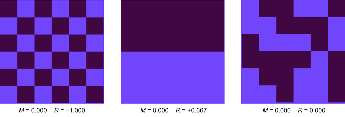
For those who want numbers rather than pictures, I offer the magnetization and local-correlation meters at the top of the program display. Magnetization is a global measure of the extent to which one color or the other dominates the lattice. Specifically, it is the number of dark cells minus the number of light cells, divided by the total number of cells:
\[M = \frac{\blacksquare - \square }{\blacksquare + \square}.\]
\(M\) ranges from \(-1\) (all light cells) through \(0\) (equal numbers of light and dark cells) to \(+1\) (all dark).
Local correlation examines all pairs of nearest-neighbor cells and tallies the number of like pairs minus the number of unlike pairs, divided by the total number of pairs:
\[R = \frac{(\square\square + \blacksquare\blacksquare) - (\square\blacksquare + \blacksquare\square) }{\square\square + \square\blacksquare + \blacksquare\square + \blacksquare\blacksquare}.\]
Again the range is from \(-1\) to \(+1\). These two quantities are both measures of order in the Ising system, but they focus on different spatial scales, global vs. local. All three of the patterns in Figure 1 have magnetization \(M = 0\), but they have very different values of local correlation \(R\).
The Ising model was invented 100 years ago by Wilhelm Lenz of the University of Hamburg, who suggested it as a thesis project for his student Ernst Ising. It was introduced as a model of a permanent magnet.
A real ferromagnet is a quantum-mechanical device. Inside, electrons in neighboring atoms come so close together that their wave functions overlap. Under these circumstances the electrons can reduce their energy slightly by aligning their spin vectors. According to the rules of quantum mechanics, an electron’s spin must point in one of two directions; by convention, the directions are labeled up and down. The ferromagnetic interaction favors pairings with both spins up or both down. Each spin generates a small magnetic dipole moment. Zillions of them acting together hold your grocery list to the refrigerator door.
In the Ising version of this structure, the basic elements are still called spins, but there is nothing twirly about them, and nothing quantum mechanical either. They are just abstract variables constrained to take on exactly two values. It really doesn’t matter whether we name the values up and down, mauve and indigo, or plus and minus. (Within the computer programs, the two values are \(+1\) and \(-1\), which means that flipping a spin is just a matter of multiplying by \(-1\).) In this article I’m going to refer to up/down spins and dark/light cells interchangeably, adopting whichever term is more convenient at the moment.
As in a ferromagnet, nearby Ising spins want to line up in parallel; they reduce their energy when they do so. This urge to match spin directions (or cell colors) extends only to nearest neighbors; more distant sites in the lattice have no influence on one another. In the two-dimensional square lattice—the setting for all my simulations—each spin’s four nearest neighbors are the lattice sites to the north, east, south, and west (including “wraparound” neighbors for cells on the boundary lines).
If neighboring spins want to point the same way, why don’t they just go ahead and do so? The whole system could immediately collapse into the lowest-energy configuration, with all spins up or all down. That does happen, but there are complicating factors and countervailing forces. Neighborhood conflicts are the principal complication: Flipping your spin to please one neighbor may alienate another. The countervailing influence is heat. Thermal fluctuations can flip a spin even when the change is energetically unfavorable.
The behavior of the Ising model is easiest to understand at the two extremities of the temperature scale. As the temperature \(T\) climbs toward infinity, thermal agitation completely overwhelms the cooperative tendencies of adjacent spins, and all possible states of the system are on an equal footing. The lattice becomes a random array of up and down spins, each of which is rapidly changing its orientation. At the opposite end of the scale, where \(T\) approaches zero, the system freezes. As thermal fluctuations subside, the spins sooner or later sink into the orderly, low-energy, fully magnetized state—although “sooner or later” can stretch out toward the age of the universe.
Things get more complicated between these extremes. Experiments with real magnets show that the transition from a hot random state to a cold magnetized state is not gradual. As the material is cooled, spontaneous magnetization appears suddenly at a critical temperature called the Curie point (about 840 K in iron). Lenz and Ising wondered whether this abrupt onset of magnetization could be seen in their simple, abstract model. Ising was able to analyze only a one-dimensional version of the system—a line or ring of spins—and he was disappointed to see no sharp phase transition. He thought this result would hold in higher dimensions as well, but on that point he was later proved wrong.
The idealized phase diagram in Figure 2 (borrowed with amendments from my 2019 article) outlines the course of events for a two-dimensional model. To the right, above the critical temperature \(T_c\), there is just one phase, in which up and down spins are equally abundant on average, although they may form transient clusters of various sizes. Below the critical point the diagram has two branches, leading to all-up and all-down states at zero temperature. As the system is cooled through \(T_c\) it must follow one branch or the other, but which one is chosen is a matter of chance.

The immediate vicinity of \(T_c\) is the most interesting region of the phase diagram. If you scroll back up to Program 1 and set the temperature near 2.27, you’ll see filigreed patterns of all possible sizes, from single pixels up to the diameter of the lattice. The time scale of fluctuations also spans orders of magnitude, with some structures winking in and out of existence in milliseconds and others lasting long enough to test your patience.
All of this complexity comes from a remarkably simple mechanism. The model makes no attempt to capture all the details of ferromagnet physics. But with minimal resources—binary variables on a plain grid with short-range interactions—we see the spontaneous emergence of cooperative, collective phenomena, as self-organizing patterns spread across the lattice. The model is not just a toy. Ten years ago Barry M. McCoy and Jean-Marie Maillard wrote:
It may be rightly said that the two dimensional Ising model… is one of the most important systems studied in theoretical physics. It is the first statistical mechanical system which can be exactly solved which exhibits a phase transition.
As I see it, the main question raised by the Ising model is this: At a specified temperature \(T\), what does the lattice of spins look like? Of course “look like” is a vague notion; even if you know the answer, you’ll have a hard time communicating it except by showing pictures. But the question can be reformulated in more concrete ways. We might ask: Which configurations of the spins are most likely to be seen at temperature \(T\)? Or, conversely: Given a spin configuration \(S\), what is the probability that \(S\) will turn up when the lattice is at temperature \(T\)?
Intuition offers some guidance on these points. Low-energy configurations should always be more likely than high-energy ones, at any finite temperature. Differences in energy should have a stronger influence at low temperature; as the system gets warmer, thermal fluctuations can mask the tendency of spins to align. These rules of thumb are embodied in a little fragment of mathematics at the very heart of the Ising model:
\[W_B = \exp\left(\frac{-E}{k_B T}\right).\]
Here \(E\) is the energy of a given spin configuration, found by scanning through the entire lattice and tallying the number of nearest-neighbor pairs that have parallel vs. antiparallel spins. In the denominator, \(T\) is the absolute temperature and \(k_B\) is Boltzmann’s constant, named for Ludwig Boltzmann, the Austrian maestro of statistical mechanics. The entire expression is known as the Boltzmann weight, and it determines the probability of observing any given configuration.
In standard physical units the constant \(k_B\) is about \(10^{-23}\) joules per kelvin, but the Ising model doesn’t really live in the world of joules and kelvins. It’s a mathematical abstraction, and we can measure its energy and temperature in any units we choose. The convention among theorists is to set \(k_B = 1\), and thereby eliminate it from the formula altogether. Then we can treat both energy and temperature as if they were pure numbers, without units.

Figure 3 confirms that the equation for the Boltzmann weight yields curves with an appropriate general shape. Lower energies correspond to higher weights, and lower temperatures yield steeper slopes. These features make the curves plausible candidates for describing a physical system such as a ferromagnet. Proving that they are not only good candidates but the unique, true description of a ferromagnet is a mathematical and philosophical challenge that I decline to take on. Fortunately, I don’t have to. The model, unlike the magnet, is a human invention, and we can make it obey whatever laws we choose. In this case let’s simply decree that the Boltzmann distribution gives the correct relation between energy, temperature, and probability.
Note that the Boltzmann weight is said to determine a probability, not that it is a probability. It can’t be. \(W_B\) can range from zero to infinity, but a probability must lie between zero and one. To get the probability of a given configuration, we need to calculate its Boltzmann weight and then divide by \(Z\), the sum of the weights of all possible configurations—a process called normalization. For a model with \(10{,}000\) spins there are \(2^{10{,}000}\) configurations, so normalization is not a task to be attempted by direct, brute-force arithmetic.
It’s a tribute to the ingenuity of mathematicians that the impossible-sounding problem of calculating \(Z\) has in fact been conquered. In 1944 Lars Onsager published a complete solution of the two-dimensional Ising model—complete in the sense that it allows you to calculate the magnetization, the energy per spin, and a variety of other properties, all as a function of temperature. I would like to say more about Onsager’s solution, but I can’t. I’ve tried more than once to work my way through his paper, but it defeats me every time. I would understand nothing at all about this result if it weren’t for a little help from my friends. Barry Cipra, in a 1987 article, and Cristopher Moore and Stephan Mertens, in their magisterial tome The Nature of Computation, rederive the solution by other means. They relate the Ising model to more tractable problems in graph theory, where I am able to follow most of the steps in the argument. Even in these lucid expositions, however, I find the ultimate result unilluminating. I’ll cite just one fact emerging from Onsager’s difficult algebraic exercise. The exact location of the critical temperature, separating the magnetic from the nonmagnetic phases, is:
\[\frac{2}{\log{(1 + \sqrt{2})}} \approx 2.269185314.\]
For those intimidated by the icy crags of Mt. Onsager, I can recommend the warm blue waters of Monte Carlo. The math is easier. There’s a clear, mechanistic connection between microscopic events and macroscopic properties. And there are the visualizations—that lively dance of the mauve and the indigo—which offer revealing glimpses of what’s going on behind the mathematical curtains. All that’s missing is exactness. Monte Carlo studies can pin down \(T_C\) to several decinal places, but they will never give the algebraic expression found by Onsager.
The Monte Carlo method was devised in the years immediately after World War II by mathematicians and physicists working at the Los Alamos Laboratory in New Mexico.
The second application was the design of nuclear weapons. The problem at hand was to understand the diffusion of neutrons through uranium and other materials. When a wandering neutron collided with an atomic nucleus, the neutron might be scattered in a new direction, or it might be absorbed by the nucleus and effectively disappear, or it might induce fission in the nucleus and thereby give rise to several more neutrons. Experiments had provided reasonable estimates of the probability of each of these events, but it was still hard to answer the crucial question: In a lump of fissionable matter with a particular shape, size, and composition, would the nuclear chain reaction fizzle or boom? The Monte Carlo method offered an answer by simulating the paths of thousands of neutrons, using random numbers to generate events with the appropriate probabilities. The first such calculations were done with the ENIAC, the vacuum-tube computer built at the University of Pennsylvania. Later the work shifted to the MANIAC, built at Los Alamos.
This early version of the Monte Carlo method is now sometimes called simple or naive Monte Carlo; I have also seen the term hit-or-miss Monte Carlo. The scheme served well enough for card games and for weapons of mass destruction, but the Los Alamos group never attempted to apply it to a problem anything like the Ising model. It would not have worked if they had tried. I know that because textbooks say so, but I had never seen any discussion of exactly how the model would fail. So I decided to try it for myself.
My plan was indeed simple and naive and hit-or-miss. First I generated a random sample of \(10{,}000\) spin configurations, drawn independently with uniform probability from the set of all possible states of the lattice. This was easy to do: I constructed the samples by the computational equivalent of tossing a fair coin to assign a value to each spin. Then I calculated the energy of each configuration and, assuming some definite temperature \(T\), assigned a Boltzmann weight. I still couldn’t convert the Boltzmann weights into true probabilities without knowing the sum of all \(2^{10{,}000}\) weights, but I could sum up the weights of the \(10{,}000\) configurations in the sample. Dividing each weight by this sum yields a relative probability: It estimates how frequently (at temperature \(T\)) we can expect to see a member of the sample relative to all the other members.
At extremely high temperatures—say \(T \gt 1{,}000\)—this procedure works pretty well. That’s because all configurations are nearly equivalent at those temperatures; they all have about the same relative probability. On cooling the system, I hoped to see a gradual skewing of the relative probabilities, as configurations with lower energy are given greater weight. What happens, however, is not a gradual skewing but a spectacular collapse. At \(T = 2\) the lowest-energy state in my sample had a relative probability of \(0.9999999979388337\), leaving just \(0.00000000206117\) to be shared among the other \(9{,}999\) members of the set.

The fundamental problem is that a small sample of randomly generated lattice configurations will almost never include any states that are commonly seen at low temperature. The histograms of Figure 4 show Boltzmann distributions at various temperatures (blue) compared with the distribution of randomly generated states (red). The random distribution is a slender peak centered at zero energy. There is slight overlap with the Boltzmann distribution at \(T = 50\), but none whatever for lower temperatures.
There’s actually some good news in this fiasco. The failure of random sampling indicates that the interesting states of the Ising system—those which give the model its distinctive behavior—form a tiny subset buried within the enormous space of \(2^{10{,}000}\) configurations. If we can find a way to focus on that subset and ignore the rest, the job will be much easier.
The means to focus more narrowly came with a second wave of Monte Carlo methods, also emanating from Los Alamos. The foundational document was a paper titled “Equation of State Calculations by Fast Computing Machines,” published in 1953. Among the five authors, Nicholas Metropolis was listed first (presumably for alphabetical reasons), and his name remains firmly attached to the algorithm presented in the paper.
With admirable clarity, Metropolis et al. explain the distinction between the old and the new Monte Carlo: “[I]nstead of choosing configurations randomly, then weighting them with \(\exp(-E/kT)\), we choose configurations with a probability \(\exp(-E/kT)\) and weight them evenly.” Starting from an arbitrary initial state, the scheme makes small, random modifications, with a bias favoring configurations with a lower energy (and thus higher Boltzmann weight), but not altogether excluding moves to higher-energy states. After many moves of this kind, the system is almost certain to be meandering through a neighborhood that includes the most probable configurations. Methods based on this principle have come to be known as MCMC, for Markov chain Monte Carlo. The Metropolis algorithm and Glauber dynamics are the best-known exemplars.
Roy Glauber also had Los Alamos connections. He worked there during World War II, in the same theory division that was home to Ulam, John von Neumann, Hans Bethe, Richard Feynman, and many other notables of physics and mathematics. But Glauber was a very junior member of the group; he was 18 when he arrived, and a sophomore at Harvard. His one paper on the Ising model was published two decades later, in 1963, and makes no mention of his former Los Alamos colleagues. It also makes no mention of Monte Carlo methods; nevertheless, Glauber dynamics has been taken up enthusiastically by the Monte Carlo community.
When applied to the Ising model, both the Metropolis algorithm and Glauber dynamics work by focusing attention on a single spin at each step, and either flipping the selected spin or leaving it unchanged. Thus the system passes through a sequence of states that differ by at most one spin flip. Statistically speaking, this procedure sounds a little dodgy. Unlike the naive Monte Carlo approach, where successive states are completely independent, MCMC generates configurations they are closely correlated. It’s a biased sample. To overcome the bias, the MCMC process has to run long enough for the correlations to fade away. With a lattice of \(N\) sites, a common protocol retains only every \(N\)th sample, discarding all those in between.
The mathematical justification for the use of correlated samples is the theory of Markov chains, devised by the Russian mathematician A. A. Markov circa 1900. It is a tool for calculating probabilities when each event depends on the previous event. And, in the Monte Carlo method, it allows one to work with those probabilities without getting bogged down in the morass of normalization.
The Metropolis and the Glauber algorithms are built on the same armature. They both rely on two main components: a visitation sequence and an acceptance function. The visitation sequence determines which lattice site to visit next; in effect, it shines a spotlight on one selected spin, proposing to flip it to the opposite orientation. The acceptance function determines whether to accept this proposal (and flip the spin) or reject it (and leave the existing spin direction unchanged). Each iteration of this two-phase process constitutes one “microstep” of the Monte Carlo procedure. Repeating the procedure \(N\) times constitutes a “macrostep.” Thus one macrostep amounts to one microstep per spin.
In the Metropolis algorithm, the visitation order is deterministic. The program sweeps through the lattice methodically, repeating the same sequence of visits in every macrostep. The original 1953 presentation of the algorithm did not prescribe any specific sequence, but the procedure was clearly designed to visit each site exactly once during a sweep. The version of the Metropolis algorithm in Program 1 adopts the most obvious deterministic option: “typewriter order.” The program chugs through the first row of the lattice from left to right, then goes through the second row in the same way, and so on down to the bottom.
Glauber dynamics takes a different approach: At each microstep the algorithm selects a single spin at random, with uniform probability, from the entire set of \(N\) spins. In other words, every spin has a \(1 / N\) chance of being chosen at each microstep, whether or not it has been chosen before. A macrostep lasts for \(N\) microsteps, but the procedure does not guarantee that every spin will get a turn during every sweep. Some sites will be passed over, while others are visited more than once. Still, as the number of steps goes to infinity, all the sites eventually get equal attention.
So much for the visitation sequence; now on to the acceptance function. It has three parts:
- Calculate \(\Delta E\), the change in energy that would result from flipping the selected spin \(s\). To determine this value, we need to examine \(s\) itself and its four nearest neighbors.
- Based on \(\Delta E\) and the temperature \(T\), calculate the probability \(p\) of flipping spin \(s\).
- Generate a random number \(r\) in the interval \([0, 1)\). If \(r \lt p\), flip the selected spin; otherwise leave it as is.
Part 2 of the acceptance rule calls for a mathematical function that maps values of \(\Delta E\) and \(T\) to a probability \(p\). To be a valid probability, \(p\) must be confined to the interval \([0, 1]\). To make sense in the context of the Monte Carlo method, the function should assign a higher probability to spin flips that reduce the system’s energy, without totally excluding those that bring an energy increase. And this preference for negative \(\Delta E\) should grow sharper as T gets lower. The specific functions chosen by the Metropolis and the Glauber algorithms satisfy both of these criteria.
Let’s begin with the Glauber acceptance function, which I’m going to call the G-rule:
\[p = \frac{e^{-\Delta E/T}}{1 + e^{-\Delta E/T}}.\]
Parts of this equation should look familiar. The expression for the Boltzmann weight, \(e^{-\Delta E/T}\), appears twice, except that the configuration energy \(E\) is replaced by \(\Delta E\), the change in energy when a specific spin is flipped.  But where the Boltzmann weight ranges from zero to infinity, the quotient of exponentials in the G-rule stays within the bounds of \(0\) to \(1\). The curve at right shows the probability distribution for \(T = 2.7\), near the critical point for the onset of magnetization. To get a qualitative understanding of the form of this curve, consider what happens when \(\Delta E\) grows without bound toward positive infinity: The numerator of the fraction goes to \(0\) while the denominator goes to \(1\), leaving a quotient that approaches \(0.0\). At the other end of the curve, as \(\Delta E\) goes to negative infinity, both numerator and denominator increase without limit, and the probability approaches (but never quite reaches) \(1.0\). Between these extremes, the curve is symmetrical and smooth. It looks like it would make a pleasant ski run.
The Metropolis acceptance criterion also includes the expression \(e^{-\Delta E/T}\), but the function and the curve are quite different. The acceptance probability is defined in a piecewise fashion:
\[p = \left\{\begin{array}{cl}
1 & \text { if } \quad \Delta E \leq 0 \\
e^{-\Delta E/T} & \text { if } \quad \Delta E>0
\end{array}\right.\]

In words, the rule says: If flipping a spin would reduce the energy of the system or leave it unchanged, always do it; otherwise, flip the spin with probability \(e^{-\Delta E/T}\). The probability curve (left) has a steep escarpment; if this one is a ski slope, it rates a black diamond. Unlike the smooth and symmetrical Glauber curve, this one has a sharp corner, as well as a strong bias. Consider a spin with \(\Delta E = 0\). Glauber flips such a spin with probability \(1/2\), but Metropolis always flips it.
The graphs in Figure 7 compare the two acceptance functions over a range of temperatures. The curves differ most at the highest temperatures, and they become almost indistinguishable at the lowest temperatures, where both curves approximate a step function. Although both functions are defined over the entire real number line, the two-dimensional Ising model allows \(\Delta E\) to take on only five distinct values: \(–8, –4, 0, +4,\) and \(+8\). Thus the Ising probability functions are never evaluated anywhere other than the positions marked by colored dots.

Here are JavaScript functions that implement a macrostep in each of the algorithms, with their differences in both visitation sequence and acceptance function:
function runMetro() {
  for (let y = 0; y < gridSize; y++) {
    for (let x = 0; x < gridSize; x++) {
      let deltaE = calcDeltaE(x, y);
      let boltzmann = Math.exp(-deltaE/temperature);
      if ((deltaE <= 0) || (Math.random() < boltzmann)) {
        lattice[x][y] *= -1;
      }
    }
  }
  drawLattice();
}

function runGlauber() {
  for (let i = 0; i < N; i++) {
    let x = Math.floor(Math.random() * gridSize);
    let y = Math.floor(Math.random() * gridSize);
    let deltaE = calcDeltaE(x, y);
    let boltzmann = Math.exp(-deltaE/temperature);
    if (Math.random() < (boltzmann / (1 + boltzmann))) {
      lattice[x][y] *= -1;
    }
  }
  drawLattice();
}
(As I mentioned above, the rest of the source code for the simuations is available on GitHub.)
We’ve seen that the Metropolis and the Glauber algorithms differ in their choice of both visitation sequence and acceptance function. They also produce different patterns or textures when you watch them in action on the computer screen. But what about the numbers? Do they predict different properties for the Ising ferromagnet?
A theorem mentioned throughout the MCMC literature says that these two algorithms (and others like them) should give identical results when properties of the model are measured at thermal equilibrium. I have encountered this statement many times in my reading, but until a few weeks ago I had never tested it for myself. Here are some magnetization data that look fairly convincing:
Magnitude of Magnetization
| T = 1.0 | T = 2.0 | T = 2.7 | T = 3.0 | T = 5.0 | T = 10.0 | |
|---|---|---|---|---|---|---|
| Metropolis | 0.9993 | 0.9114 | 0.0409 | 0.0269 | 0.0134 | 0.0099 |
| Glauber | 0.9993 | 0.9118 | 0.0378 | 0.0274 | 0.0136 | 0.0100 |
The table records the absolute value of the magnetization in Metropolis and Glauber simulations at various temperatures. Five of the six measurements differ by less than \(0.001\); the exception cames at \(T = 2.7\), near the critical point, where the difference rises to about \(0.003\). Note that the results are consistent with the presence of a phase transition: Magnetization remains close to \(0\) down to the critical point and then approaches \(1\) at lower temperatures. (By reporting the magnitude, or absolute value, of the magnetization, we treat all-up and all-down states as equivalent.)
I made the measurements by first setting the temperature and then letting the simulation run for at least 1,000 macrosteps in order to reach an equilibrium condition.
When I first looked at these results and saw the close match between Metropolis and Glauber, I felt a twinge of paradoxical surprise. I call it paradoxical because I knew before I started what I would see, and that’s exactly what I did see, so obviously I should not have been surprised at all. But some part of my mind didn’t get that memo, and as I watched the two algorithms converge to the same values all across the temperature scale, it seemed remarkable.
The theory behind this convergence was apparently understood by the pioneers of MCMC in the 1950s. The theorem states that any MCMC algorithm will produce the same distribution of states at equilibrium, as long as the algorithm satisfies two conditions, called ergodicity and detailed balance.
Both algorithms also exhibit detailed balance, which is essentially a requirement of reversibility. Suppose that while watching a model run, you observe a transition from state \(A\) to state \(B\). Detailed balance says that if you continue observing long enough, you will see the inverse transition \(B \rightarrow A\) with the same frequency as \(A \rightarrow B\). Given the shapes of the acceptance curves, this assertion may seem implausible. If \(A \rightarrow B\) is energetically favorable, then \(B \rightarrow A\) must be unfavorable, and it will have a lower probability. But there’s another factor at work here. Remember we are assuming the system is in equilibrium, which implies that the occupancy of each state—or the amount of time the system spends in that state—is proportional to the state’s Boltzmann weight. Because the system is more often found in state \(B\), the transition \(B \rightarrow A\) has more chances to be chosen, counterbalancing the lower intrinsic probability.
The claim that Metropolis and Glauber yield identical results applies only when the Ising system is in equilibrium—poised at the eternal noon where the sun stands still and nothing ever changes. For Metropolis and his colleagues at Los Alamos in the early 1950s, understanding the equilibrium behavior of a computational model was challenge enough. They were coaxing answers from a computer with about four kilobytes of memory. Ten years later, however, Glauber wanted to look beyond equilibrium. For example, he wanted to know what happens when the temperature suddenly changes. How do the spins reorganize themselves during the transient period between one equilibrium state and another? He designed his version of the Ising model specifically to deal with such dynamic situations. He wrote in his 1963 paper:
If the mathematical problems of equilibrium statistical mechanics are great, they are at least relatively well-defined. The situation is quite otherwise in dealing with systems which undergo large-scale changes with time…. We have attempted, therefore, to devise a form of the Ising model whose behavior can be followed exactly, in statistical terms, as a function of time.

Clearly, in this dynamic situation, the algorithms are not identical or interchangeable. The Metropolis program adapts more quickly to the cooler environment; Glauber produces a slower but steadier rise in magnetization. The curves differ in shape, with Metropolis exhibiting a distinctive “knee” where the slope flattens. I want to know what causes these differences, but before digging into that question it seems important to understand why both algorithms are so agonizingly slow. At the right edge of the graph the blue Metropolis curve is approaching the equilibrium value of magnetization (which is about 0.91), but it has taken 7,500 Monte Carlo macrosteps (or 75 million microsteps) to get there. The red Glauber curve will require many more. What’s the holdup?
To put this sluggishness in perspective, let’s look at the behavior of local spin correlations measured under the same circumstances. Graphing the average nearest-neighbor correlation following a sudden temperature drop produces these hockey-stick curves:

The response is dramatically faster; both algorithms reach quite high levels of local correlation within just a few macrosteps.
For a hint of why local correlations grow so much faster than global magnetization, it’s enough to spend a few minutes watching the Ising simulation evolve on the computer screen. When the temperature plunges from warm \(T = 5\) to frigid \(T = 2\), nearby spins have a strong incentive to line up in parallel, but magnetization does not spread uniformly across the entire lattice. Small clusters of aligned spins start expanding, and they merge with other clusters of the same polarity, thereby growing larger still. It doesn’t take long, however, before clusters of opposite polarity run into one another, blocking further growth for both. From then on, magetization is a zero-sum game: The up team can win only if the down team loses.
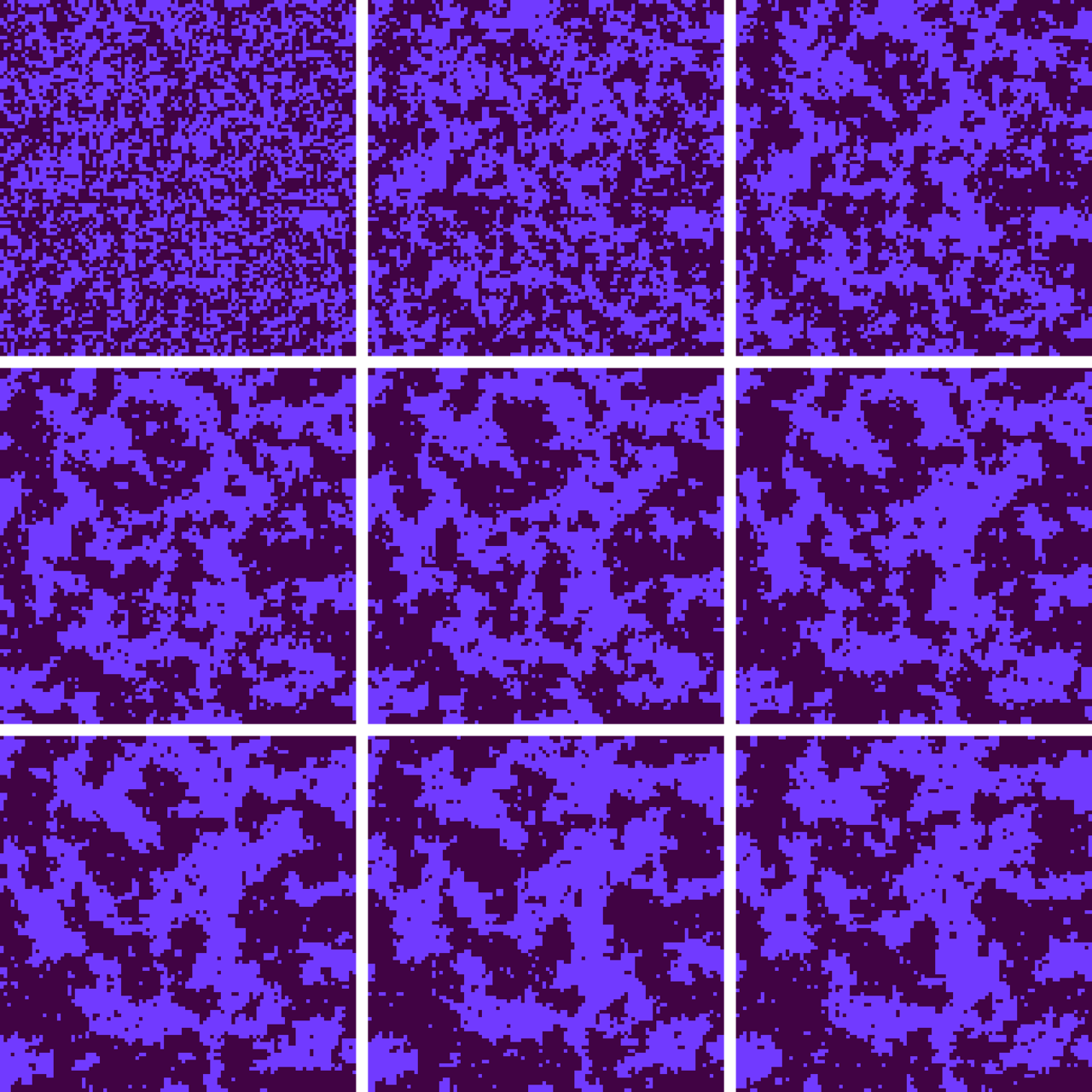
Figure 10 shows the first few Monte Carlo macrosteps following a flash freeze. The initial configuration at the upper left reflects the high-temperature state, with a nearly random, salt-and-pepper mix of up and down spins. The rest of the snapshots (reading left to right and top to bottom) show the emergence of large-scale order. Prominent clusters appear after the very first macrostep, and by the second or third step some of these blobs have grown to include hundreds of lattice sites. But the rate of change becomes sluggish thereafter. The balance of power may tilt one way and then the other, but it’s hard for either side to gain a permanent advantage. The mottled, camouflage texture will persist for hundreds or thousands of steps.
If you choose a single spin at random from such a mottled lattice, you’ll almost surely find that it lives in an area where most of the neighbors have the same orientation. Hence the high levels of local correlation. But that fact does not imply that the entire array is approaching unanimity. On the contrary, the lattice can be evenly divided between up and down domains, leaving a net magnetization near zero. (Yes, it’s like political polarization, where homogeneous states add up to a deadlocked nation.)
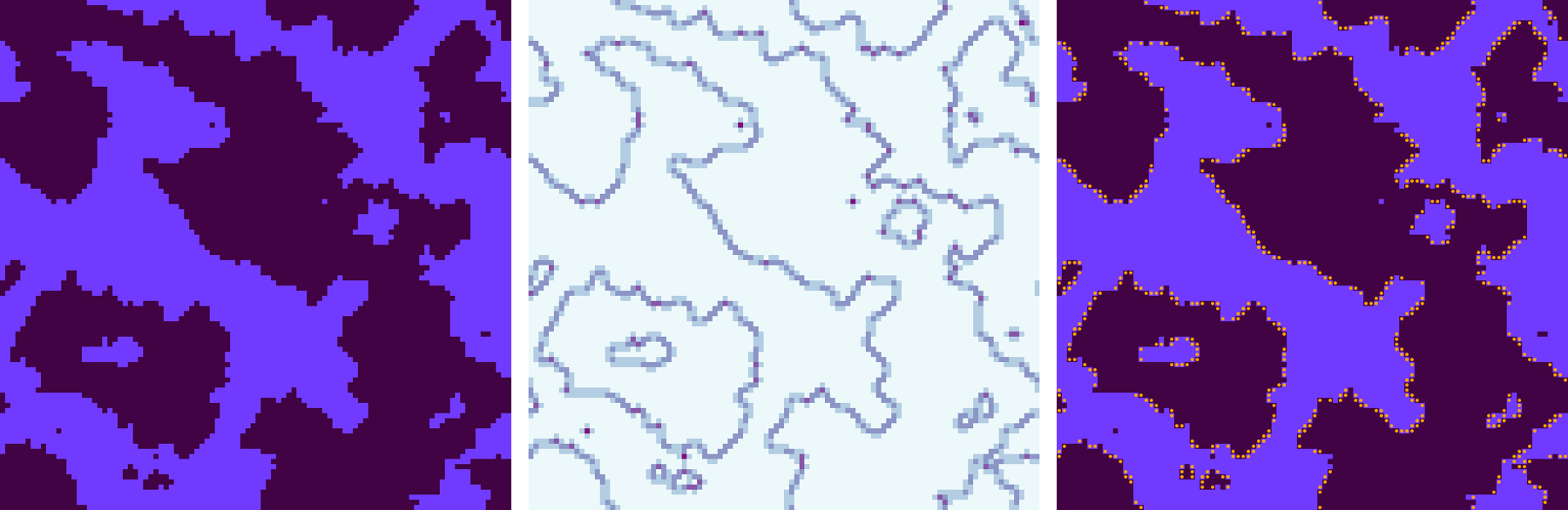
The images in Figure 11 show three views of the same state of an Ising lattice. At left is the conventional representation, with sinuous, interlaced territories of nearly pure up and down spins. The middle panel shows the same configuration recolored according to the local level of spin correlation. The vast majority of sites (lightest hue) are surrounded by four neighbors of the same orientation; they correspond to both the mauve and the indigo regions of the leftmost image. Only along the boundaries between domains is there any substantial conflict, where darker colors mark cells whose neighbors include spins of the opposite orientation. The panel at right highlights a special category of sites—those with exactly two parallel and two antiparallel neighbors. They are special because they are tiny neutral territories wedged between the contending factions. Flipping such a spin does not alter its correlation status; both before and after it has two like and two unlike neighbors. Flipping a neutral spin also does not alter the total energy of the system. But it can shift the magnetization. Indeed, flipping such “neutral” spins is the main agent of evolution in the Ising system at low temperature.
The struggle to reach full magnetization in an Ising lattice looks like trench warfare. Contending armies, almost evenly matched, face off over the boundary lines between up and down territories. All the action is along the borders; nothing that happens behind the lines makes much difference. Even along the boundaries, some sections of the front are static. If a domain margin is a straight line parallel to the \(x\) or \(y\) axis, the sites on each side of the border have three friendly neighbors and only one enemy; they are unlikely to flip. The volatile neutral sites that make movement possible appear only at corners and along diagonals, where neighborhoods are evenly split.
From these observations and ruminations I feel I’ve acquired some intuition about why my Monte Carlo simulations bog down during the transition from a chaotic to an ordered state. But why is the Glauber algorithm even slower than the Metropolis?
Since the schemes differ in two features—the visitation sequence and the acceptance function—it makes sense to investigate which of those features has the greater effect on the convergence rate. That calls for another computational experiment.
The tableau below is a mix-and-match version of the MCMC Ising simulation. In the control panel you can choose the visitation order and the acceptance function independently. If you select a deterministic visitation order and the M-rule acceptance function, you have the classical Metropolis algorithm. Likewise random order and the G-rule correspond to Glauber dynamics. But you can also pair deterministic order with the G-rule or random order with the M-rule. (The latter mixed-breed choice is what I unthinkingly implemented in my 2019 program.)
I have also included an acceptance rule labeled M*, which I’ll explain below.
Watching the screen while switching among these alternative components reveals that all the combinations yield different visual textures, at least at some temperatures. Also, it appears there’s something special about the pairing of deterministic visitation order with the M-rule acceptance function (i.e., the standard Metropolis algorithm).
Try setting the temperature to 2.5 or 3.0. I find that the distinctive sensation of fluttery motion—bird flocks migrating across the screen—appears only with the deterministic/M-rule combination. With all other pairings, I see amoeba-like blobs that grow and shrink, fuse and divide, but there’s not much coordinated motion.
Now lower the temperature to about 1.5, and alternately click Run and Reset until you get a persistent bold stripe that crosses the entire grid either horizontally or vertically.
These observations suggest some curious interactions between the visitation order and the acceptance function, but they do not reveal which factor gives the Metropolis algorithm its speed advantage. Using the same program, however, we can gather some statistical data that might help answer the question.

These curves were a surprise to me. From my earlier experiments I already knew that the Metropolis algorithm—the combination of elements in the blue curve—would outperform the Glauber version, corresponding to the red curve. But I expected the acceptance function to account for most of the difference. The data do not support that supposition. On the contrary, they suggest that both elements matter, and the visitation sequence may even be the more important one. A deterministic visitation order beats a random order no matter which acceptance function it is paired with.
My expectations were based mainly on discussions of the “mixing time” for various Monte Carlo algorithms. Mixing time is the number of steps needed for a simulation to reach equilibrium from an arbitrary initial state, or in other words the time needed for the system to lose all memory of how it began. If you care only about equilibrium properties, then an algorithm that offers the shortest mixing time is likely to be preferred, since it also minimizes the number of CPU cycles you have to waste before you can start taking data. Discussions of mixing time tend to focus on the acceptance function, not the visitation sequence. In particular, the M-rule acceptance function of the Metropolis algorithm was explicitly designed to minimize mixing time.
What I am measuring in my experiments is not exactly mixing time, but it’s closely related. Going from an arbitrary initial state to equilibrium at a specified temperature is much like a transition from one temperature to another. What’s going on inside the model is similar. Thus if the acceptance function determines the mixing time, I would expect it also to be the major factor in adapting to a new temperature regime.
On the other hand, I can offer a plausible-sounding theory of why visitation order might matter. The deterministic model scans through all \(10{,}000\) lattice sites during every Monte Carlo macrostep; each such sweep is guaranteed to visit every site exactly once. The random order makes no such promise. In that algorithm, each microstep selects a site at random, whether or not it has been visited before. A macrostep concludes after \(10{,}000\) such random choices. Under this protocol some sites are passed over without being selected even once, while others are chosen two or more times. How many sites are likely to be missed? During each microstep, every site has the same probability of being chosen, namely \(1 / 10{,}000\). Thus the probability of not being selected on any given turn is \(9{,}999 / 10{,}000\). For a site to remain unvisited throughout an entire macrostep, it must be passed over \(10{,}000\) times in a row. The probability of that event is \((9{,}999 / 10{,}000)^{10{,}000}\), which works out to about \(0.368\).
Excluding more than a third of the sites on every pass through the lattice seems certain to have some effect on the outcome of an experiment. In the long run the random selection process is fair, in the sense that every spin is sampled at the same frequency. But the rate of convergence to the equilibrium state may well be lower.
There are also compelling arguments for the importance of the acceptance function. A key fact mentioned by several authors is that the M acceptance rule leads to more spin flips per Monte Carlo step. If the energy change of a proposed flip is favorable or neutral, the M-rule always approves the flip, whereas the G-rule rejects some proposed flips even when they lower the energy. Indeed, for all values of \(T\) and \(\Delta E\) the M-rule gives a higher probability of acceptance than the G-rule does. This liberal policy—if in doubt, flip—allows the M-rule to explore the space of all possible spin configurations more rapidly.
The discrete nature of the Ising model, with just five possible values of \(\Delta E\), introduces a further consideration. At \(\Delta E = \pm 4\) and at \(\Delta E = \pm 8\), the M-rule and the G-rule don’t actually differ very much when the temperature is below the critical point (see Figure 7). The two curves diverge only at \(\Delta E = 0\): The M-rule invariably flips a spin in this circumstance, whereas the G-rule does so only half the time, assigning a probability of \(0.5\). This difference is important because the lattice sites where \(\Delta E = 0\) are the ones that account for almost all of the spin flips at low temperature. These are the neutral sites highlighted in the right panel ofFigure 11, the ones with two like and two unlike neighbors.
This line of thought leads to another hypothesis. Maybe the big difference between the Metropolis and the Glauber algorithms has to do with the handling of this single point on the acceptance curve. And there’s an obvious way to test the hypothesis: Simply change the M-rule at this one point, having it toss a coin whenever \(\Delta E = 0\). The definition becomes:
\[p = \left\{\begin{array}{cl}
1 & \text { if } \quad \Delta E \lt 0 \\
\frac{1}{2} & \text { if } \quad \Delta E = 0 \\
e^{-\Delta E/T} & \text { if } \quad \Delta E>0
\end{array}\right.\]
This modified acceptance function is the M* rule offered as an option in Program 2. Watching it in action, I find that switching the Metropolis algorithm from M to M* robs it of its most distinctive traits: At high temperature the fluttering birds are banished, and at low temperature the wiggling worms are immobilized. The effects on convergence rates are also intriguing. In the Metropolis algorithm, replacing M with M* greatly diminishes convergence speed, from a standout level to just a little better than average. At the same time, in the Glauber algorithm replacing G with M* brings a considerable performance improvement; when combined with random visitation order, M* is superior not only to G but also to M.

I don’t know how to make sense of all these results except to suggest that both the visitation order and the acceptance function have important roles, and non-additive interactions between them may also be at work. Here’s one further puzzle. In all the experiments described above, the Glauber algorithm and its variations respond to a disturbance more slowly than Metropolis. But before dismissing Glauber as the perennial laggard, take a look at Figure 14.

Here we’re observing a transition from low to high temperature, the opposite of the situation discussed above. When going in this direction—from an orderly phase to a chaotic one, melting rather than freezing—both algorithms are quite zippy, but Glauber is a little faster than Metropolis. Randomness, it appears, is good for randomization. That sounds sensible enough, but I can’t explain in any detail how it comes about.
Up to this point, a deterministic visitation order has always meant the typewriter scan of the lattice—left to right and top to bottom. Of course this is not the only deterministic route through the grid. In Program 3 you can play with a few of the others.
Why should visitation order matter at all? As long as you touch every site exactly once, you might imagine that all sequences would produce the same result at the end of a macrostep. But it’s not so, and it’s not hard to see why. Whenever two sites are neighbors, the outcome of applying the Monte Carlo process can depend on which neighbor you visit first.
Consider the cruciform configuration at right. At first glance, you might assume that the dark central square will be unlikely to change its state.  After all, the central square has four like-colored neighbors; if it were to flip, it would have four opposite-colored neighbors, and the energy associated with those spin-spin interactions would rise from \(-4\) to \(+4\). Any visitation sequence that went first to the central square would almost surely leave it unflipped. However, when the Metropolis algorithm comes tap-tap-tapping along in typewriter mode, the central cell does in fact change color, and so do all four of its neighbors. The entire structure is annihilated in a single sweep of the algorithm. (The erased pattern does leave behind a ghost—one of the diagonal neighbor sites flips from light to dark. But then that solitary witness disappears on the next sweep.)
To understand what’s going on here, just follow along as the algorithm marches from left to right and top to bottom through the lattice. When it reaches the central square of the cross, it has already visited (and flipped) the neighbors to the north and to the west. Hence the central square has two neighbors of each color, so that \(\Delta E = 0\). According to the M-rule, that square must be flipped from dark to light. The remaining two dark squares are now isolated, with only light neighbors, so they too flip when their time comes.
The underlying issue here is one of chronology—of past, present, and future. Each site has its moment in the present, when it surveys its surroundings and decides (based on the results of the survey) whether or not to change its state. But in that present moment, half of the site’s neighbors are living in the past—the typewriter algorithm has already visited them—and the other half are in the future, still waiting their turn.
A well-known alternative to the typewriter sequence might seem at first to avoid this temporal split decision. Superimposing a checkerboard pattern on the lattice creates two sublattices that do not communicate for purposes of the Ising model. Each black square has only white neighbors, and vice versa. Thus you can run through all the black sites (in any order; it really doesn’t matter), flipping spins as needed. Afterwards you turn to the white sites. These two half-scans make up one macrostep. Throughout the process, every site sees all of its neighbors in the same generation. And yet time has not been abolished. The black cells, in the first half of the sweep, see four neighboring sites that have not yet been visited. The white cells see neighbors that have already had their chance to flip. Again half the neighbors are in the past and half in the future, but they are distributed differently.
There are plenty of other deterministic sequences. You can trace successive diagonals; in Program 3 they run from southwest to northeast. There’s the ever-popular boustrophedonic order, following in the footsteps of the ox in the plowed field. More generally, if we number the sites consecutively from \(1\) to \(10{,}000\), any permutation of this sequence represents a valid visitation order, touching each site exactly once. There are \(10{,}000!\) such permutations, a number that dwarfs even the \(2^{10{,}000}\) configurations of the binary-valued lattice. The permuted choice in Program 3 selects one of those permutations at random; it is then used repeatedly for every macrostep until the program is reset. The re-permuted option is similar but selects a new permutation for each macrostep. The random selection is here for comparison with all the deterministic variations.
(There’s one final button labeled simultaneous, which I’ll explain below. If you just can’t wait, go ahead and press it, but I won’t be held responsible for what happens.)
The variations add some further novelties to the collection of curious visual effects seen in earlier simulations. The fluttering wings are back, in the diagonal as well as the typewriter sequences. Checkerboard has a different rhythm; I am reminded of a crowd of frantic commuters in the concourse of Grand Central Terminal. Boustrophedon is bidirectional: The millipede’s legs carry it both up and down or both left and right at the same time. Permuted is similar to checkerboard, but re-permuted is quite different.
The next question is whether these variant algorithms have any quantitative effect on the model’s dynamics. Figure 15 shows the response to a sudden freeze for seven visitation sequences. Five of them follow roughly the same arcing trajectory. Typewriter remains at the top of the heap, but checkerboard, diagonal, boustrophedon, and permuted are all close by, forming something like a comet tail. The random algorithm is much slower, which is to be expected given the results of earlier experiments.

The intriguing case is the re-permuted order, which seems to lie in the no man’s land between the random and the deterministic algorithms. Perhaps it belongs there. In earlier comparisons of the Metropolis and Glauber algorithms, I speculated that random visitation is slower to converge because many sites are passed over in each macrostep, while others are visited more than once. That’s not true of the re-permuted visitation sequence, which calls on every site exactly once, though in random order. The only difference between the permuted algorithm and the re-permuted one is that the former reuses the same permutation over and over, whereas re-permuted creates a new sequence for every macrostep. The faster convergence of the static permuted algorithm suggests there is some advantage to revisiting all the same sites in the same order, no matter what that order may be. Most likely this has something to do with sites that get switched back and forth repeatedly, on every sweep.
Now for the mysterious simultaneous visitation sequence. If you have not played with it yet in Program 3, I suggest running the following experiment. Select the typewriter sequence, press the Run button, reduce the temperature to 1.10 or 1.15, and wait until the lattice is all mauve or all indigo, with just a peppering of opposite-color dots. (If you get a persistent wide stripe instead of a clear field, raise the temperature and try again.) Now select the simultaneous visitation order.
This behavior is truly weird but not inexplicable. The algorithm behind it is one that I have always thought should be the best approach to a Monte Carlo Ising simulation. In fact it seems to be just about the worst.
All of the other visitation sequences are—as the term suggests they should be—sequential. They visit one site at a time, and differ only in how they decide where to go next. If you think about the Ising model as if it were a real physical process, this kind of serialization seems pretty implausible. I can’t bring myself to believe that atoms in a ferromagnet politely take turns in flipping their spins. And surely there’s no central planner of the sequence, no orchestra conductor on a podium, pointing a baton at each site when its turn comes.
Natural systems have an all-at-onceness to them. They are made up of many independent agents that are all carrying out the same kinds of activities at the same time. If we could somehow build an Ising model out of real atoms, then each cell or site would be watching the state of its four neighbors all the time, and also sensing thermal agitation in the lattice; it would decide to flip whenever circumstances favored that choice, although there might be some randomness to the timing. If we imagine a computer model of this process (yes, a model of a model), the most natural implementation would require a highly parallel machine with one processor per site.
Lacking such fancy hardware, I make due with fake parallelism. The simultaneous algorithm makes two passes through the lattice on every macrostep. On the first pass, it looks at the neighborhood of each site and decides whether or not to flip the spin, but it doesn’t actually make any changes to the lattice. Instead, it uses an auxiliary array to keep track of which spins are scheduled to flip. Then, after all sites have been surveyed in the first pass, the second pass goes through the lattice again, flipping all the spins that were designated in the first pass. The great advantage of this scheme is that it avoids the temporal oddities of working within a lattice where some spins have already been updated and others have not. In the simultaneous algorithm, all the spins make the transition from one generation to the next at the same instant.
When I first wrote a program to implement this scheme, almost 40 years ago, I didn’t really know what I was doing, and I was utterly baffled by the outcome. The information mechanics group at MIT (Ed Fredkin, Tommaso Toffoli, Norman Margolus, and Gérard Vichniac) soon came to my rescue and explained what was going on, but all these years later I still haven’t quite made my peace with it.
What continues to disturb me about this phenomenon is that I still think the simultaneous update rule is in some sense more natural or realistic than many of the alternatives. It is closer to how the world works—or how I imagine that it works—than any serial ordering of updates. Yet nature does not create magnets that continually swing between states that have the highest possible energy. (A 2002 paper by Gabriel Pérez, Francisco Sastre, and Rubén Medina attempts to rehabilitate the simultaneous-update scheme, but the blinking catastrophe remains pretty catastrophic.)
This is not the only bizarre behavior to be found in the dark corners of Monte Carlo Ising models. In the Metropolis algorithm,  simply setting the temperature to a very high value (say, \(T = 1{,}000\)) has a similar effect. Again every spin flips on every cycle, producing a display that throbs violently but otherwise remains unchanged. The explanation is laughably simple. At high temperature the Metropolis acceptance function flattens out and yields a spin-flip probability near \(1\) for all sites, no matter what their neighborhood looks like. The Glauber acceptance curve also flattens out, but at a value of 0.5, which leads to a totally randomized lattice—a more plausible high-temperature outcome.
I have not seen this high-temperature anomaly mentioned in published works on the Metropolis algorithm, although it must have been noticed many times over the years. Perhaps it’s not mentioned because this kind of failure will never be seen in physical systems. \(T = 1{,}000\) in the Ising model is \(370\) times the critical temperature; the corresponding temperature in iron would be over \(300{,}000\) kelvins. Iron boils at \(3{,}000\) kelvins.
The curves in Figure 15 and most of the other graphs above are averages taken over hundreds of repetitions of the Monte Carlo process. The averaging operation is meant to act like sandpaper, smoothing out noise in the curves, but it can also grind away interesting features, replacing a population of diverse individuals with a single homogenized exemplar. Figure 17 shows six examples of the lumpy and jumpy trajectories recorded during single runs of the program:

In these squiggles, magnetization does not grow smoothly or steadily with time. Instead we see spurts of growth followed by plateaus and even episodes of retreat. One of the Metropolis runs is slower than the three Glauber examples, and indeed makes no progress toward a magnetized state. Looking at these plots, it’s tempting to explain them away by saying that the magnetization measurements exhibit high variance. That’s certain true, but it’s not the whole story.
Figure 18 shows the distribution of times needed for a Metropolis Ising model to reach a magnetization of \(0.85\) in response to a sudden shift from \(T = 10\) to \(T= 2\). The histogram records data from \(10{,}000\) program runs, expressing convergence time in Monte Carlo macrosteps.

The median of this distribution is \(451\) macrosteps; in other words, half of the runs concluded in \(451\) steps or fewer. But the other half of the population is spread out over quite a wide range. Runs of \(10\) times the median length are not great rareties, and the blip at the far right end of the \(x\) axis represents the \(59\) runs that had still not reached the threshold after \(10{,}000\) macrosteps (where I stopped counting). This is a heavy-tailed distribution, which appears to be made up of two subpopulations. In one group, forming the sharp peak at the left, magnetization is quick and easy, but members of the other group are recalcitrant, holding out for thousands of steps. I have a hypothesis about what distinguishes those two sets. The short-lived ones are ponds; the stubborn ones that overstay their welcome are rivers.
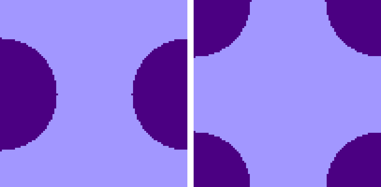
When an Ising system cools and becomes fully magnetized, it goes from a salt-and-pepper array of tiny clusters to a monochromatic expanse of one color or the other. At some point during this process, there must be a moment when the lattice is divided into exactly two regions, one light and one dark. 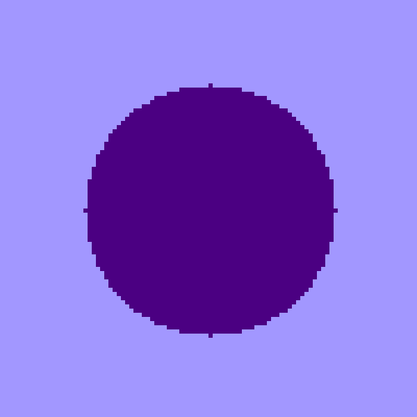 Figure 19 shows one possible configuration: A pond of indigo cells lies within a mauve landmass that covers the rest of the lattice. If the system is to make further progress toward full magnetization, either the pond must dry up (leaving a blank expanse of mauve), or the pond must overflow its banks, inundating the remaining land area (leaving a sea of indigo). Experiments reveal that the former outcome is overwhelmingly more likely. Why? One guess is that it’s just a matter of majority rule: Whichever patch controls the greater amount of territory will eventually prevail. But that’s not it. Even when the pond covers most of the lattice, leaving only a thin strip of shoreline at the edges, the surrounding land eventually squeezes the pond out of existence.
I believe the correct answer has to do with the concepts of inside and outside, connected and disconnected, open sets and closed sets—but I can’t articulate these ideas in a way that would pass mathematical muster. I want to say that the indigo pond is a bounded region, entirely enclosed by the unbounded mauve continent. But the wraparound lattice make it hard to wrap your head around this notion. The two images in Figure 20 show exactly the same object as Figure 19, the only difference being that the origin of the coordinate system has moved, so that the center of the disk seems to lie on an edge or in a corner of the lattice. The indigo pond is still surrounded by the mauve continent, but it sure doesn’t look that way. In any case, why should boundedness determine which area survives the Monte Carlo process?
For me, the distinction between inside and outside began to make sense when I tried taking a more “local” view of the boundaries between regions, and the curvature of those boundaries. As noted in connection with Figure 11, boundaries are places where you can expect to find neutral lattice sites (i.e., \(\Delta E = 0\)), which are the only sites where a spin is likely to change orientation at low temperature.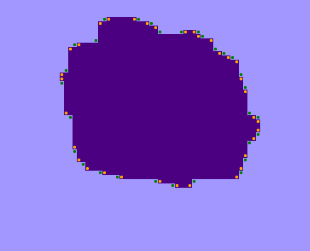 In honor of their neutrality I’m going to call these sites Swiss cells. In Figure 21 I have marked all the Swiss cells with colored dots (making them dotted Swiss!). Orange-dotted cells lie in the indigo interior of the pond, whereas green dots lie outside on the mauve landmass.
I’ll spare you the trouble of counting the dots in Figure 21: There are 34 orange ones inside the pond but only 30 green ones outside. That margin could be significant. Because the dotted cells are likely to change state, the greater abundance of orange dots means there are more indigo cells ready to turn mauve than mauve cells that might become indigo. If the bias continues as the system evolves, the indigo region will steadily lose area and eventually be swallowed up.
But is there any reason to think the interior of the pond will always have a surplus of neutral sites susceptible to flipping? 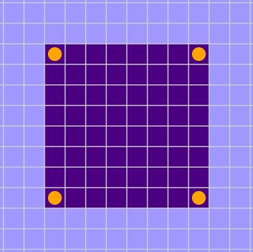 The simplest geometry for a pond is a square or rectangle, as in Figure 22. It has four interior Swiss cells (in the corners) and no exterior Swiss cells—which would be marked with green dots if they existed. In other words, no mauve cells along the outside boundary of a square or rectangular pond have exactly two mauve and two indigo neighbors.
What if the shape becomes a little more complicated? Perhaps the square pond grows a protuberance on one side, and an invagination on another, as in Figure 23. 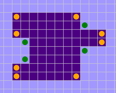 Each of these modifications generates a pair of orange-dotted neutral sites inside the patch, along with a pair of green-dotted ones outside. Thus the count of inside minus outside remains unchanged at four. On first noticing this invariance I had a delicious Aha! moment. There’s a conservation law, I thought. No matter how you alter the outline of the pond, the neutral sites inside will outnumber those outside by four.
This notion is not utterly crazy. If you walk clockwise around the boundary of the simple square pond in Figure 22, you will have made four right turns by the time you get back to your starting point. Each of those right turns creates a neutral cell in the interior of the pond—we’ll call them innie turns—where you can place an orange dot. A clockwise circuit of the modified pond in Figure 23, with its excrenscences and increscences, requires some left turns as well as right turns. 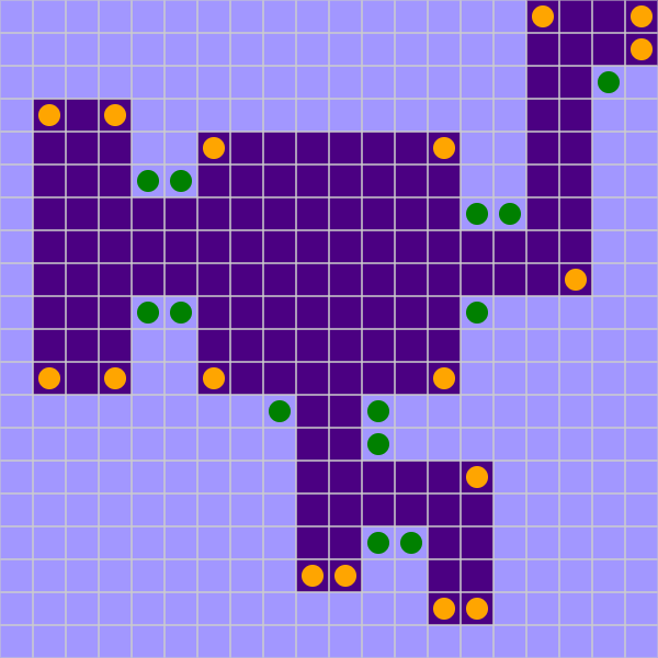 Each left turn produces a neutral cell in the mauve exterior region—it’s an outie turn—earning a green dot. But for every outie turn added to the perimeter, you’ll have to make an additional innie turn in order to get back to your starting point. Thus, except for the four original corners, innie and outie turns are like particles and antiparticles, always created and annihilated in pairs. A closed path, no matter how convoluted, always has exactly four more innies than outies. The four-turn differential is again on exhibit in the more elaborate example of Figure 24, where the orange dots prevail 17 to 13. Indeed, I assert that there are always four more innie turns than outie turns on the perimeter of any simple (i.e., non-self-intersecting) closed curve on the square lattice. (I think this is one of those statements that is obviously true but not so simple to prove, like the claim that every simple closed curve on the plane has an inside and an outside.)
Unfortunately, even if the statement about counting right and left turns is true, the corresponding statement about orange and green dots is not. 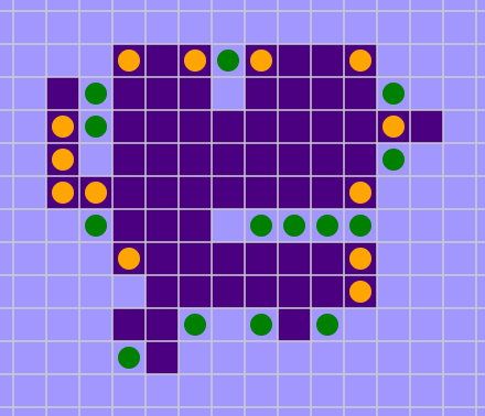 It holds only for a rather special subclass of lattice shapes, namely those in which the perimeter line not only has no self-intersections but never comes within one lattice spacing of itself. In effect, we exclude all closed figures that have hair on their surface or pores in their skin. Figure 25 shows an example of a shape that violates the rule. Narrow, single-lane passages create neutral sites that do not come in matched innie/outie pairs. In this case there are more green dots than orange ones, which might be taken to suggest that the indigo area will grow rather than shrink.
In my effort to explain why ponds always evaporate, I seem to have reached a dead end. I should have known from the outset that the effort was doomed. I can’t prove that ponds always shrink because they don’t. The system is ergodic: Any state can be reached from any other state in a finite number of steps. In particular, a single indigo cell (a very small pond) can grow to cover the whole lattice. The sequence of steps needed to make that happen is improbable, but it certainly exists.
If proof is out of reach, maybe we can at least persuade ourselves that the pond shrinks with high probability. And we have a tool for doing just that: It’s called the Monte Carlo method. Figure 26 follows the fate of a \(25 \times 25\) square pond embedded in an otherwise blank lattice of \(100 \times 100\) sites, evolving under Glauber dynamics at a very low temperature \((T = 0.1)\). The uppermost curve, in indigo, shows the steady evaporation of the pond, dropping from the original \(625\) sites to \(0\) after about \(320\) macrosteps. The middle traces record the abundance of Swiss sites, orange for those inside the pond and green for those outside. Because of the low temperature, these are the only sites that have any appreciable likelihood of flipping. The black trace at the bottom is the difference between orange and green. For the most part it hovers at \(+4\), never exceeding that value but seldom falling much below it, and making only one brief foray into negative territory. Statistically speaking, the system appears to vindicate the innie/outie hypothesis. The pond shrinks because there are almost always more flippable spins inside than outside.

Figure 26 is based on a single run of the Monte Carlo algorithm. Figure 27 presents essentially the same data averaged over \(1{,}000\) Monte Carlo runs under the same conditions—starting with a \(25 \times 25\) square pond and applying Glauber dynamics at \(T = 0.1\).

The pond’s loss of area follows a remarkably linear path, with a steady rate very close to two lattice sites per Monte Carlo macrostep. And it’s clear that virtually all of these pondlike blocks of indigo cells disappear within a little more than \(300\) macrosteps, putting them in the tall peak at the short end of the lifetime distribution in Figure 18. None of them contribute to the long tail that extends out past \(10{,}000\) steps.
So much for the quick-drying ponds. What about the long-flowing rivers?
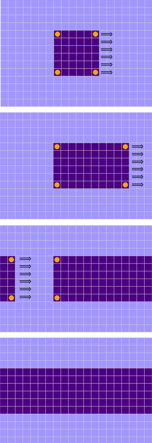 We can convert a pond into a river. Take a square block of dark pixels and tug on one side, stretching the square into an elongated rectangle. When the moving side of the rectangle reaches the edge of the lattice, just keep on pulling. Because of the model’s wraparound boundary conditions, the lattice actually has no edge; when an object exits to the right, it immediately re-enters on the left. Thus you can keep pulling the (former) right side of the rectangle until it meets up with the (former) left side.
When the two sides join, everything changes. It’s not just a matter of adjusting the shape and size of the rectangle. There is no more rectangle! By definition, a rectangle has four sides and four right-angle corners. The object now occupying the lattice has only two sides and no corners. It may appear to have corners at the far left and right, but that’s an artifact of drawing the figure on a flat plane. It really lives on a torus, and the band of indigo cells is like a ring of chocolate icing that goes all the way around the doughnut. Or it’s a river—an endless river. You can walk along either bank as far as you wish, and you’ll never find a place to cross.
The topological difference between a pond and a river has dire consequences for Monte Carlo simulations of the Ising model. When the rectangle’s four corners disappeared, so did the four orange dots marking interior Swiss cells. Indeed, the river has no neutral cells at all, neither inside nor outside. At temperatures near zero, where neutral cells are the only ones that ever change state, the river becomes an all-but-eternal feature. The Monte Carlo process has no effect on it. The system is stuck in a metastable state, with no practical way to reach the lower-energy state of full magnetization.
When I first noticed how a river can block magnetization, I went looking to see what others might have written about the phenomonon. I found nothing. There was lots of talk about metastability in general, but none of the sources I consulted mentioned this particular topological impediment. I began to worry that I had made some blunder in programming or had misinterpreted what I was seeing. Finally I stumbled on a 2002 paper by Spirin, Krapivsky, and Redner that reports essentially the same observations and extends the discussion to three dimensions, where the problem is even worse.
A river with perfectly straight banks looks rather unnatural—more like a canal.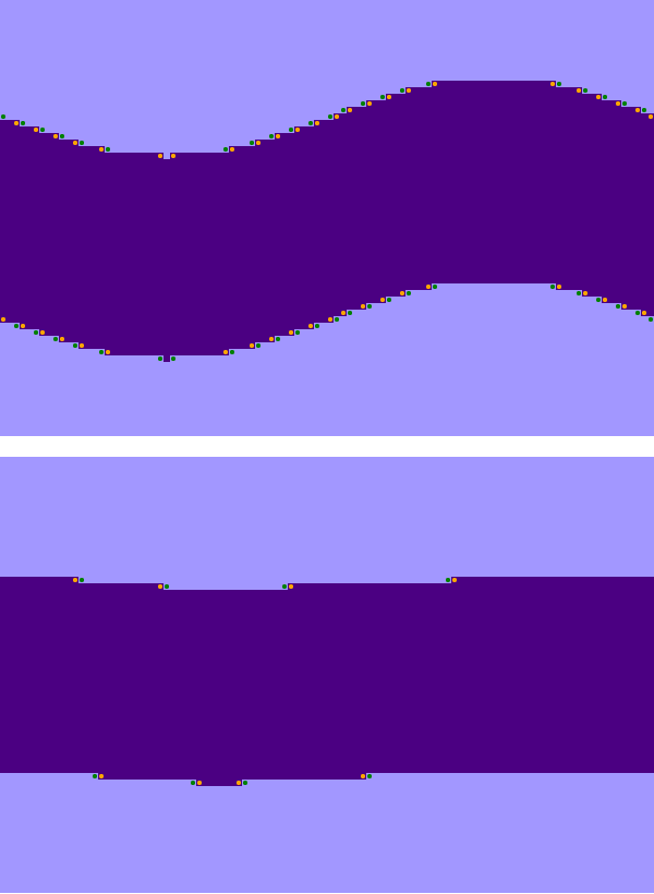 Perhaps adding some meanders would make a difference in the outcome? The upper part of Figure 29 shows a river with a sinusoidal bend. The curves create 46 interior neutral cells and an exactly equal number of exterior ones. These corner points serve as handholds where the Monte Carlo process can get a grip, so one might hope that by flipping some of these spins the channel will narrow and eventually close.
But that’s not what happens. The lower part of Figure 29 shows the same stretch of river after \(1{,}000\) Monte Carlo macrosteps at \(T = 0.1\). The algorithm has not amplified the sinuosity; on the contrary, it has shaved off the peaks and filled in the troughs, generally flattening the terrain. After \(5{,}000\) steps the river has returned to a perfectly straight course. No neutral cells remain, so no further change can be expected in any human time frame.
The presence or absence of four corners makes all the difference between ponds and rivers. Ponds shrink because the corners create a consistent bias: Sites subject to flipping are more numerous inside than outside, which means, over the long run, that the outside steadily encroaches on the inside’s territory. That bias does not exist for rivers, where the number of interior and exterior neutral sites is equal on average. Figure 30 records the inside-minus-outside difference for the first \(1{,}000\) steps of a simulation beginning with a sinusoidal river.

The difference hovers near zero, though with short-lived excursions both above and below; the mean value is \(+0.062\).
Even at somewhat higher temperatures, any pattern that crosses from one side of the grid to the other will stubbornly resist extinction. Figure 31 shows snapshots every \(1{,}000\) macrosteps in the evolution of a lattice at \(T = 1.0\), which is well below the critical temperature but high enough to allow a few energetically unfavorable spin flips. The starting configuration was a sinusoidal river, but by \(1{,}000\) steps it has already become a thick, lumpy band. In subsequent snapshots the ribbon grows thicker and thinner, migrates up and down—and then abruptly disappears, sometime between the \(8{,}000\)th and the \(9{,}000\)th macrostep.
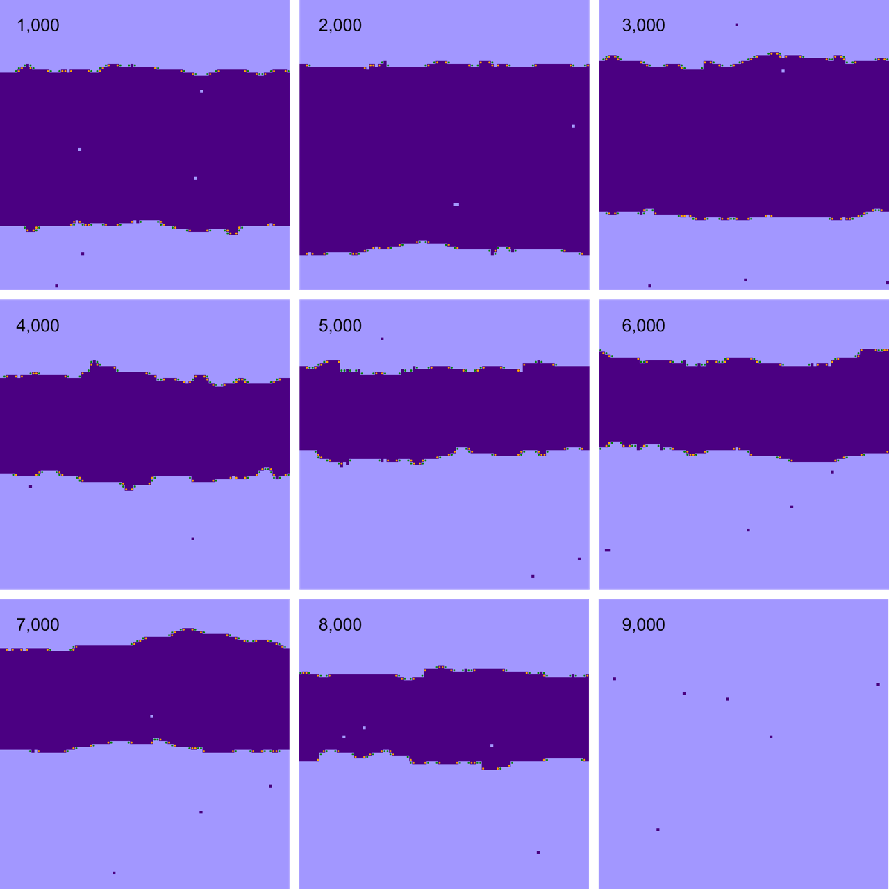
Swiss cells, with equal numbers of friends and enemies among their neighbors, appear wherever a boundary line takes a turn. All the rest of the sites along a boundary—on both sides—have three friendly neighbors and one enemy neighbor. At a site of this kind, flipping a spin carries an energy penalty of \(\Delta E = +4\). At \(T = 1.0\) the probability of such an event is roughly \(1/50\). In a \(10{,}000\)-site lattice crossed by a river there can be as many as \(200\) of these three-against-one sites, so we can expect to see a few of them flip during every macrostep. Thus at \(T = 1.0\) the river is not a completely static formation, as it is at temperatures closer to zero. The channel can shift or twist, grow wider or narrower. But these motions are glacially slow, not only because they depend on somewhat rare events but also because the probabilities are unbiased. At every step the river is equally likely to grow wider or narrower; on average, it goes nowhere.
In one last gesture to support my claim that short-lived patterns are ponds and long-lived patterns are rivers I offer Figure 32:

A troubling question is whether these uncrossable rivers that block full magnetization in Ising models also exist in physical ferromagnets. It seems unlikely. The rivers I describe above owe their existence to the models’ wraparound boundary conditions. The crystal lattices of real magnetic materials do not share that topology. Thus it seems that metastability may be an artifact or a mere incidental feature of the model, not something present in nature.
Statistical mechanics is generally formulated in terms of systems without boundaries. You construct a theory of \(N\) particles, but it’s truly valid only in the “thermodynamic limit,” where \(N \to \infty\). Under this regime the two-dimensional Ising model would be studied on a lattice extending over an infinite plane. Computer models can’t do that, and so we wind up with tricks like wraparound boundary conditions, which can be considered a hack for faking infinity.
It’s a pretty good hack. As in an infinite lattice, every site has the same local environment, with exactly four neighbors, who also have four neighbors, and so on. There are no edges or corners that require special treatment. For these reasons wraparound or periodic boundary conditions have always been the most popular choice for computational models in the sciences, going back at least as far as 1953. Still, there are glitches. If you were standing on a wraparound lattice, you could walk due north forever, but you’d keep passing your starting point again and again. If you looked into the distance, you’d see the back of your own head. For the Ising model, perhaps the most salient fact is this: On a genuinely infinite plane, every simple, finite, closed curve is a pond; no finite structure can behave like a river, transecting the entire surface so that you can’t get around it. Thus the wraparound model differs from the infinite one in ways that may well alter important conclusions.
These defects are a little worrisome. On the other hand, physical ferromagnets are also mere finite approximations to the unbounded spaces of thermodynamic theory. A single magnetic domain might have \(10^{20}\) atoms, which is large compared with the \(10^4\) sites in the models presented here, but it’s a long ways short of infinity. The domains have boundaries, which can have a major influence on their properties. All in all, it seems like a good idea to explore the space of possibile boundary conditions, including some alternatives to the wraparound convention. Hence Program 4:
An extra row of cells around the perimeter of the lattice serves to make the boundary conditions visible in this simulation. The cells in this halo layer are not active participants in the Ising process; they serve as neighbors to the cells on the periphery of the lattice, but their own states are not updated by the Monte Carlo algorithm. To mark their special role, their up and down states are indicated by red and pink instead of indigo and mauve.
The behavior of wraparound boundaries is already familiar. If you examine the red/pink stripe along the right edge of the grid, you will see that it matches the leftmost indigo/mauve column. Similar relations determine the patterns along the other edges.
The two simplest alternatives to the wraparound scheme are static borders made up of cells that are always up or always down. You can probably guess how they will affect the outcome of the simulation. Try setting the temperature around 1.5 or 2.0, then click back and forth between all up and all down as the program runs. The border color quickly invades the interior space, encircling a pond of the opposite color and eventually squeezing it down to nothing. Switching to the opposite border color brings an immediate re-enactment of the same scene with all colors reversed. The biases are blatant.
Another idea is to assign the border cells random values, chosen independently and with equal probability. A new assignment is made after every macrostep. Randomness is akin to high temperature, so this choice of boundary condition amounts to an Ising lattice surrounded by a ring of fire. There is no bias in favor of up or down, but the stimulation from the sizzling periphery creates recurrent disturbances even at temperatures near zero, so the system never attains a stable state of full magnetization.
Before I launched this project, my leading candidate for a better boundary condition was a zero border. This choice is equivalent to an “open” or “free” boundary, or to no boundary at all—a universe that just ends in blankness. Implementing open boundaries is slightly irksome because cells on the verge of nothingness require special handling: Those along the edges have only three neighbors, and those in the corners only two. A zero boundary produces the same effect as a free boundary without altering the neighbor-counting rules. The cells of the outer ring all have a numerical value of \(0\), indicated by gray. For the interior cells with numerical values of \(+1\) and \(-1\), the zero cells act as neighbors without actually contributing to the \(\Delta E\) calculations that determine whether or not a spin flips.
The zero boundary introduces no bias favoring up or down, it doesn’t heat or cool the system, and it doesn’t tamper with the topology, which remains a simple square embedded in a flat plane. Sounds ideal, no? However, it turns out the zero boundary has a lot in common with wraparound borders. In particular, it allows persistent rivers to form—or maybe I should call them lakes. I didn’t see this coming before I tried the experiment, but it’s not hard to understand what’s happening. On the wraparound lattice, elongating a rectangle until two opposite edges meet eliminates the Swiss cells at the four corners. The same thing happens when a rectangle extends all the way across a lattice with zero borders. The corner cells, now up against the border, no longer have two friendly and two enemy neighbors; instead they have two friends, one enemy, and one cel of spin zero, for a net \(\Delta E\) of \(+1\).
A pleasant surprise of these experiments was the boundary type I have labeled sampled. The idea is to make the boundary match the statistics of the interior of the lattice, but without regard to the geometry of any patterns there. For each border cell \(b\) we select an interior cell \(s\) at random, and assign the color of \(s\) to \(b\). The procedure is repeated after each macrostep. The border therefore maintains the same up/down proportion as the interior lattice, and always favors the majority. If the spins are evenly split between mauve and indigo, the border region shows no bias; as soon as the balance begins to tip, however, the border shifts in the same direction, supporting and hastening the trend.
If you tend to root for the underdog, this rule is not for you—but we can turn it upside down, assigning a color opposite that of a randomly chosen interior cell. The result is interesting. Magnetization is held near \(0\), but at low temperature the local correlation coefficient approaches \(1\). The lattice devolves into two large blobs of no particular shape that circle the ring like wary wrestlers, then eventually reach a stable truce in which they split the territory either vertically or horizontally. This behavior has no obvious bearing on ferromagnetism, but maybe there’s an apt analogy somewhere in the social or political sciences.
The curves in Figure 33 record the response to a sudden temperature step in systems using each of six boundary conditions. The all-up and all-down boundaries converge the fastest—which is no surprise, since they put a thumb on the scale. The response of the sampled boundary is also quick, reflecting its weathervane policy of supporting the majority. The random and zero boundaries are the slowest; they follow identical trajectories, and I don’t know why. Wraparound is right in the middle of the pack. All of these results are for Glauber dynamics, but the curves for the Metropolis algorithm are very similar.

The menu in Program 4 has one more choice, labeled twisted. I wrote the code for this one in response to the question, “I wonder what would happen if…?” Twisted is the same as wraparound, except that one side is given a half-twist before it is mated with the opposite edge. Thus if you stand on the right edge near the top of the lattice and walk off to the right, you will re-enter on the left near the bottom. The object formed in this way is not a torus but a Klein bottle—a “nonorientable surface without boundary.” All I’m going to say about running an Ising model on this surface is that the results are not nearly as weird as I expected. See for yourself.
I have one more toy to present for your amusement: the MCMC microscope. It was the last program I wrote, but it should have been the first.
All of the programs above produce movies with one frame per macrostep. In that high-speed, high-altitude view it can be hard to see how individual lattice sites are treated by the algorithm. The MCMC microscope provides a slo-mo close-up, showing the evolution of a Monte Carlo Ising system one microstep at a time. The algorithm proceeds from site to site (in an order determined by the visitation sequence) and either flips the spin or not (according to the acceptance function).
As the algorithm proceeds, the site currently under examination is marked by a hot-pink outline. Sites that have yet to be visited are rendered in the usual indigo or mauve; those that have already had their turn are shown in shades of gray. The Microstep button advances the algorithm to the next site (determined by the visitation sequence) and either flips the spin or leaves it as-is (according to the acceptance function). The Macrostep button performs a full sweep of the lattice and then pauses; the Run button invokes a continuing series of microsteps at a somewhat faster pace. Some adjustments to this protocol are needed for the simultaneous update option. In this mode no spins are changed during the scan of the lattice, but those that will change are marked with a small square of constrasting gray. At the end of the macrostep, all the changes are made at once.
The Dotted Swiss checkbox paints orange and green dots on neutral cells (those with equal numbers of friendly and enemy neighbors). Doodle mode allows you to draw on the lattice via mouse clicks and thereby set up a specific initial pattern.
I’ve found it illuminating to draw simple geometric figures in doodle mode, then watch as they are transformed and ultimately destroyed by the various algorithms. These experiments are particularly interesting with the Metropolis algorithm at very low temperature. Under these conditions the Monte Carlo process—despite its roots in randomness—becomes very nearly deterministic. Cells with \(\Delta E \le 0\) always flip; other cells never do. (What, never? Well, hardly ever.) Thus we can speak of what happens when a program is run, rather than just describing the probability distribution of possible outcomes.
Here’s a recipe to try: Set the temperature to its lower limit, choose doodle mode, down initialization, typewriter visitation, and the M-rule acceptance function. Now draw some straight lines on the grid in four orientations: vertical, horizontal, and along both diagonals. Each line can be six or seven cells long, but don’t let them touch. Lines in three of the four orientations are immediately erased when the program runs; they disappear after the first macrostep. The one survivor is the diagonal line oriented from lower left to upper right, or southwest to northeast. With each macrostep the line migrates one cell to the left, and also loses one site at the bottom. This combination of changes gives the subjective impression that the pattern is moving not only left but also upward. I’m pretty sure that this phenomenon is responsible for the fluttering wings illusion seen at much higher temperatures (and higher animation speeds).
If you perform the same experiment with the diagonal visitation order, you’ll see exactly the same outcomes. A question I can’t answer is whether there is any pattern that serves to discriminate between the typewriter and diagonal orders. What I’m seeking is some arrangement of indigo cells on a mauve background that I could draw on the grid and then look away while you ran one algorithm or the other for some fixed number of macrosteps (which I get to specify). Afterwards, I win if I can tell which visitation sequence you chose.
The checkerboard algorithm is also worth trying with the four line orientations. The eventual outcome is the same, but the intermediate stages are quite different.
Finally I offer a few historical questions that seem hard to settle, and some philosophical musings on what it all means.
How did the method get the name “Monte Carlo”?
The name, of course, is an allusion to the famous casino, a prodigious producer and consumer of randomness. Nicholas Metropolis claimed credit for coming up with the term. In a 1987 retrospective he wrote:
It was at that time [spring of 1947] that I suggested an obvious name for the statistical method—a suggestion not unrelated to the fact that Stan [Ulam] had an uncle who would borrow money from relatives because he “just had to go to Monte Carlo.”
An oddity of this story is that Metropolis was not at Los Alamos in 1947. He left after the war and didn’t return until 1948.
Ulam’s account of the matter does not contradict the Metropolis version,
It seems to me that the name Monte Carlo contributed very much to the popularization of this procedure. It was named Monte Carlo because of the element of chance, the production of random numbers with which to play the suitable games.
Note the anonymous passive voice: “It was named…,” with no hint of by whom. If Ulam was so carefully noncommittal, who am I to insist on a definite answer?
As far as I know, the phrase “Monte Carlo method” first appeared in public print in 1949, in an article co-authored by Metropolis and Ulam. Presumably the term was in use earlier among the denizens of the Los Alamos laboratory. Daniel McCracken, in a 1955 Scientific American article, said it was a code word invented for security reasons. This is not implausible. Code words were definitely a thing at Los Alamos (the place itself was designated “Project Y”), but I’ve never seen the code word status of “Monte Carlo” corroborated by anyone with first-hand knowledge.
Who invented the Metropolis algorithm?
To raise the question, of course, is to hint that it was not Metropolis.
The 1953 paper that introduced Markov chain Monte Carlo, “Equation of State Calculations by Fast Computing Machines,” had five authors, who were listed in alphabetical order: Nicholas Metropolis, Arianna W. Rosenbluth, Marshall N. Rosenbluth, Augusta H. Teller, and Edward Teller. The two Rosenbluths were wife and husband, as were the two Tellers. Who did what in this complicated collaboration? Apparently no one thought to ask that question until 2003, when J. E. Gubernatis of Los Alamos was planning a symposium to mark the 50th anniversary of MCMC. He got in touch with Marshall Rosenbluth, who was then in poor health. Nevertheless, Rosenbluth attended the gathering, gave a talk, and sat for an interview. (He died a few months later.)
According to Rosenbluth, the basic idea behind MCMC—sampling the states of a system according to their Boltzmann weight, while following a Markov chain from one state to the next—came from Edward Teller. Augusta Teller wrote a first draft of a computer program to implement the idea. Then the Rosenbluths took over. In particular, it was Arianna Rosenbluth who wrote the program that produced all the results reported in the 1953 paper. Gubernatis adds:
Marshall’s recounting of the development of the Metropolis algorithm first of all made it very clear that Metropolis played no role in its development other than providing computer time.
In his interview, Rosenbluth was even blunter: “Metropolis was boss of the computer laboratory. We never had a single scientific discussion with him.”
These comments paint a rather unsavory portrait of Metropolis as a credit mooch. I don’t know to what extent that harsh verdict might be justified. In his own writings, Metropolis makes no overt claims about his contributions to the work. On the other hand, he also makes no disclaimers; he never suggests that someone else’s name might be more appropriately attached to the algorithm.
An interesting further question is who actually wrote the 1953 paper—who put the words together on the page. Internal textual evidence suggests there were at least two writers. Halfway through the article there’s a sudden change of tone, from gentle exposition to merciless technicality.
In recent years the algorithm has acquired the hyphenated moniker Metropolis-Hastings, acknowledging the contributions of W. Keith Hastings, a Canadian mathematician and statistician. Hastings wrote a 1970 paper that generalized the method, showing it could be applied to a wider class of problems, with probability distributions other than Boltzmann’s. Hastings is also given credit for rescuing the technique from captivity among the physicists and bringing it home to statistics, although it was another 20 years before the statistics community took much notice.
I don’t know who started the movement to name the generalized algorithm “Metropolis-Hastings.” The hyphenated term was already fairly well established by 1995, when Siddhartha Chib and Edward Greenberg put it in the title of a review article.
Who invented Glauber dynamics?
In this case there is no doubt or controversy about authorship. Glauber wrote the 1963 paper, and he did the work reported in it. On the other hand, Glauber did not invent the Monte Carlo algorithm that now goes by the name “Glauber dynamics.” His aim in tackling the Ising model was to find exact, mathematical solutions, in the tradition of Ising and Onsager. (Those two authors are the only ones cited in Glauber’s paper.) He never mentions Monte Carlo methods or any other computational schemes.
So who did devise the algorithm? The two main ingredients—the G-rule and the random visitation sequence—were already on the table in the 1950s. A form of the G-rule acceptance function \(e^{-\Delta E/T} / (1 + e^{-\Delta E/T})\) was proposed in 1954 by John G. Kirkwood of Yale University, a major figure in statistical mechanics at midcentury. He suggested it to the Los Alamos group as an alternative to the M-rule. Although the suggestion was not taken, the group did acknowledge that it would produce valid simulations. The random visitation sequence was used in a followup study by the Los Alamos group in 1957. (By then the group was led by William W. Wood, who had been a student of Kirkwood.)
Those two ingredients first came together a few years later in work by P. A. Flinn and G. M. McManus, who were then at Westinghouse Research in Pittsburgh. Their 1961 paper describes a computer simulation of an Ising model with both random visitation order and the \(e^{-\Delta E/T} / (1 + e^{-\Delta E/T})\) acceptance function, two years before Glauber’s article appeared. On grounds of publication priority, shouldn’t the Monte Carlo variation be named for Flinn and McManus rather than Glauber?
For a while, it was. There were dozens of references to Flinn and McManus throughout the 1960s and 70s. For example, an article by G. W. Cunningham and P. H. E. Meijer compared and evaluated the two main MCMC methods, identifying them as algorithms introduced by “Metropolis et al.” and by “Flinn and McManus.” A year later another compare-and-contrast article by John P. Valleau and Stuart G. Whittington adopted the same terminology. Neither of these articles mentions Glauber.
According to Semantic Scholar, the phrase “Glauber dynamics” first appeared in the physics literature in 1977, in an article by Ph. A. Martin. But this paper is a theoretical work, with no computational component, along the same lines as Glauber’s own investigation. Among the Semantic Scholar listings, “Glauber dynamics” was first mentioned in the context of Monte Carlo studies by A. Sadiq and Kurt Binder, in 1984. After that, the balance shifted strongly toward Glauber.
In bringing up the disappearance of Flinn and McManus from the Ising and Monte Carlo literature, I don’t mean to suggest that Glauber doesn’t deserve his recognition. His main contribution to studies of the Ising model—showing that it could give useful results away from equilibrium—is of the first importance. On the other hand, attaching his name to a Monte Carlo algorithm is unhelpful. If you turn to his 1963 paper to learn about the origin of the algorithm, you’ll be disappointed.
One more oddity. I have been writing the G-rule as
\[\frac{e^{-\Delta E/T}}{1 + e^{-\Delta E/T}},\]
which is the way it appeared in Flinn and McManus, as well as in many recent accounts of the algorithm. However, nothing resembling this expression is to be found in Glauber’s paper. Instead he defined the rule in terms of the hyperbolic tangent. Reconstructing various bits of his mathematics in a form that could serve as a Monte Carlo acceptance function, I come up with:
\[\frac{1}{2}\left(1 -\tanh \frac{\Delta E}{2 T}\right).\]
The two expressions are mathematically synonymous, but the prevalence of the first form suggests that some authors who cite Glauber rather than Flinn and McManus are not getting their notation from the paper they cite.
Who made the first pictures of an Ising lattice?
When I first heard of the Ising model, sometime in the 1970s, I would read statements along the lines of “as the system cools to the critical temperature, fluctuations grow in scale until they span the entire lattice.” I wanted to see what that looked like. What kinds of patterns or textures would appear, and how they would evolve over time? In those days, live motion graphics were too much to ask for, but it seemed reasonable to expect at least a still image, or perhaps a series of them covering a range of temperatures.
In my reading, however, I found no pictures. Part of the reason was surely technological. Turning computations into graphics wasn’t so easy in those days. But I suspect another motive as well. A computational scientist who wanted to be taken seriously was well advised to focus on quantitative results. A graph of magnetization as a function of temperature was worth publishing; a snapshot of a single lattice configuration might seem frivolous—not real physics but a plaything like the Game of Life. Nevertheless, I still yearned to see what it would look like.
In 1979 I had an opportunity to force the issue. I was working with Kenneth G. Wilson, a physicist then at Cornell University, on a Scientific American article about “Problems in Physics with Many Scales of Length.” The problems in question included the Ising model, and I asked Wilson if he could produce pictures showing spin configurations at various temperatures. He resisted; I persisted; a few weeks later I received a fat envelope of fanfold paper, covered in arrays of \(1\)s and \(0\)s. With help from the Scientific American art department the numbers were transformed into black and white squares:
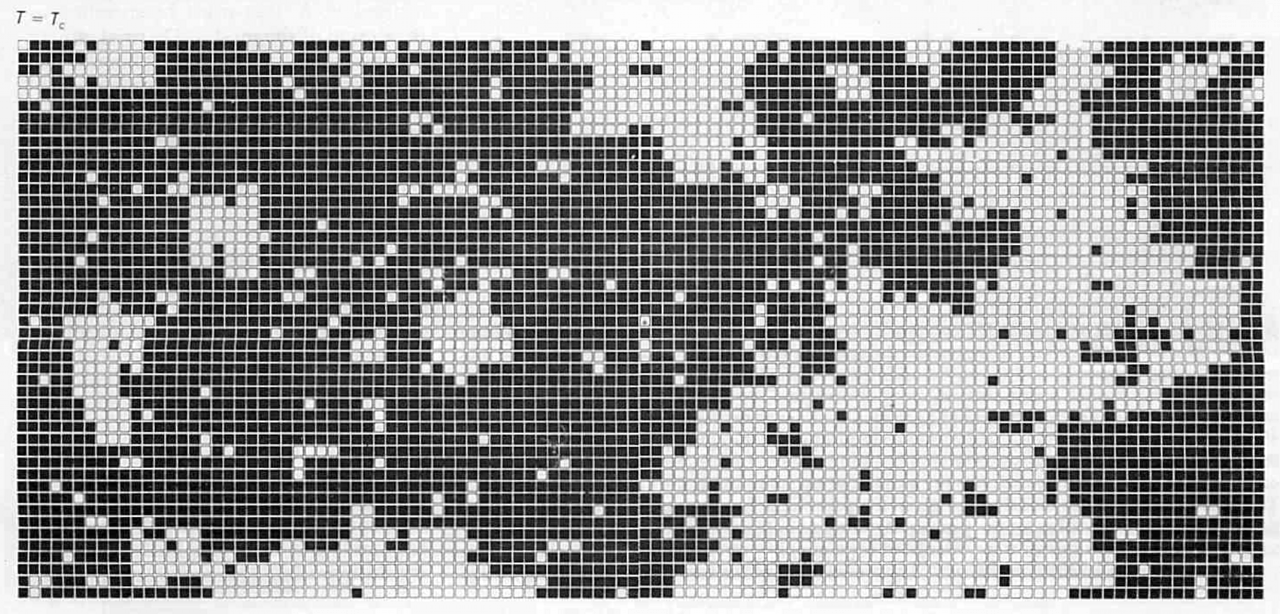
This particular image, one of three we published, is at the critical temperature. Wilson credited his colleagues Stephen Shenker and Jan Tobochnik for writing the program that produced it.
The lattice pictures made by Wilson, Shenker, and Tobochnik were the first I had ever seen of an Ising model at work, but they were not the first to be published. In recent weeks I’ve discovered a 1974 paper by P. A. Flinn in which black-and-white spin tableaux form the very centerpiece of the presentation. Flinn discusses aspects of the appearance of these grids that would be very hard to reduce to simple numerical facts:
Phase separation may be seen to occur by the formation and growth of clusters, but they look rather more like “seaweed” than like the roughly round clusters of traditional theory. The structures look somewhat like those observed in phase-separated glass.
I also found one even earlier instance of lattice diagrams, in a 1963 paper by J. R. Beeler, Jr., and J. A. Delaney. Are they the first?
What does the Ising model model?
Modeling calls for a curious mix of verisimilitude and fakery. A miniature steam locomotive chugging along the tracks of a model railroad reproduces in meticulous detail the pistons and linkage rods that drive the wheels of the real locomotive. But in the model it’s the wheels that impart motion to the links and pistons, not the other way around. The model’s true power source is hidden—an electric motor tucked away inside, where the boiler ought to be.
Scientific models also rely on shortcuts and simplifications. In a physics textbook you will meet the ideal gas, the frictionless pendulum, the perfectly elastic spring, the falling body that encounters no air resistance, the planet whose entire mass is concentrated at a dimensionless point. Such idealizations are not necessarily defects. By brushing aside irrelevant details, a good model allows a deeper truth to shine through. The problem, of course, is that some details are not irrelevant.
The Ising model is a fascinating case study in this process. Lenz and Ising set out to explain ferromagnetism, and almost all later discussions of the model (including the one you are reading right now) put some emphasis on that connection. The original aim was to find the simplest framework that would exhibit important properties of real ferromagnets, most notably the sudden onset of magnetization at the Curie temperature. As far as I can tell, the Ising model has failed in this respect. Some of the omitted details were of the essence; quantum mechanics just won’t go away, no matter how much we might like it to. These days, serious students of magnetism seem to have little interest in simple grids of flipping spins. A 2006 review of “modeling, analysis, and numerics of ferromagnetism,” by Martin Kružík and Andreas Prohl, doesn’t even mention the Ising model.
Yet the model remains wildly popular, the subject of hundreds of papers every year. Way back in 1967, Stephen G. Brush wrote that the Ising model had become “the preferred basic theory of all cooperative phenomena.” I’d go even further. I think it’s fair to say the Ising model has become an object of study for its own sake. The quest is to understand the phase diagram of the Ising system itself, whether or not it tells us anything about magnets or other physical phenomena.
Uprooting the Ising system from its ancestral home in physics leaves us with a model that is not a model of anything. It’s like a map of an imaginary territory; there is no ground truth. You can’t check the model’s accuracy by comparing its predictions with the results of experiments.
Seeing the Ising model as a free-floating abstraction, untethered from the material world, is a prospect I find exhilarating. We get to make our own universe—and we’ll do it right this time, won’t we! However, losing touch with physics is also unsettling. On what basis are we to choose between versions of the model, if not through fidelity to nature? Are we to be guided only by taste or convenience? A frequent argument in support of Glauber dynamics is that it seems more “natural” than the Metropolis algorithm. I would go along with that judgment: The random visitation sequence and the smooth, symmetrical curve of the G-rule both seem more like something found in nature than the corresponding Metropolis apparatus. But does naturalness matter if the model is solely a product of human imagination?
Further Reading
Bauer, W. F. 1958. The Monte Carlo method. Journal of the Society for Industrial and Applied Mathematics 6(4):438–451.
http://www.cs.fsu.edu/~mascagni/Bauer_1959_Journal_SIAM.pdf
Beeler, J. R. Jr., and J. A. Delaney. 1963. Order-disorder events produced by single vacancy migration. Physical Review 130(3):962–971.
Binder, Kurt. 1985. The Monte Carlo method for the study of phase transitions: a review of some recent progress. Journal of Computational Physics 59:1–55.
Binder, Kurt, and Dieter W. Heermann. 2002. Monte Carlo Simulation in Statistical Physics: An Introduction. Fourth edition. Berlin: Springer-Verlag.
Brush, Stephen G. 1967. History of the Lenz-Ising model. Reviews of Modern Physics 39:883-893.
Chib, Siddhartha, and Edward Greenberg. 1995. Understanding the Metropolis-Hastings Algorithm. The American Statistician 49(4): 327–335.
Cipra, Barry A. 1987. An introduction to the Ising model. American Mathematical Monthly 94:937-959.
Cunningham, G. W., and P. H. E. Meijer. 1976. A comparison of two Monte Carlo methods for computations in statistical mechanics. Journal Of Computational Physics 20:50-63.
Davies, E. B. 1982. Metastability and the Ising model. Journal of Statistical Physics 27(4):657–675.
Diaconis, Persi. 2009. The Markov chain Monte Carlo revolution. Bulletin of the American Mathematical Society 46(2):179–205.
Eckhardt, R. 1987. Stan Ulam, John von Neumann, and the Monte Carlo method. Los Alamos Science 15:131–137.
Flinn, P. A., and G. M. McManus. 1961. Monte Carlo calculation of the order-disorder transformation in the body-centered cubic lattice. Physical Review 124(1):54–59.
Flinn, P. A. 1974. Monte Carlo calculation of phase separation in a two-dimensional Ising system. Journal of Statistical Physics 10(1):89–97.
Fosdick, L. D. 1963. Monte Carlo computations on the Ising lattice. Methods in Computational Physics 1:245–280.
Geyer, Charles J. 2011. Intorduction to Markov chain Monte Carlo. In Handbook of Markov Chain Monte Carlo, edited by Steve Brooks, Andrew Gelman, Galin Jones and Xiao-Li Meng, pp. 3–48. Boca Raton: Taylor & Francis.
Glauber, R. J., 1963. Time-dependent statistics of the Ising model. Journal of Mathematical Physics 4:294–307.
Gubernatis, James E. (editor). 2003. The Monte Carlo Method in the Physical Sciences: Celebrating the 50th Anniversary of the Metropolis Algorithm. Melville, N.Y.: American Institute of Physics.
Halton, J. H. 1970. A retrospective and prospective survey of the Monte Carlo method. SIAM Review 12(1):1–63.
Hammersley, J. M., and D. C. Handscomb. 1964. Monte Carlo Methods. London: Chapman and Hall.
Hastings, W. K. 1970. Monte Carlo sampling methods using Markov chains and their applications. Biometrika 57(1):97–109.
Hayes, Brian. 2000. Computing science: The world in a spin. American Scientist, Vol. 88, No. 5, September-October 2000, pages 384-388. http://bit-player.org/bph-publications/AmSci-2000-09-Hayes-Ising.pdf
Hitchcock, David B. 2003. A history of the Metropolis–Hastings algorithm. The American Statistician 57(4):254–257. https://doi.org/10.1198/0003130032413
Hurd, Cuthbert C. 1985. A note on early Monte Carlo computations and scientific meetings. Annals of the History of Computing 7(2):141–155.
Ising, Ernst. 1925. Beitrag zur Theorie des Ferromagnetismus. Zeitschrift für Physik 31:253–258.
Janke, Wolfhard, Henrik Christiansen, and Suman Majumder. 2019. Coarsening in the long-range Ising model: Metropolis versus Glauber criterion. Journal of Physics: Conference Series, Volume 1163, International Conference on Computer Simulation in Physics and Beyond 24–27 September 2018, Moscow, Russian Federation. https://iopscience.iop.org/article/10.1088/1742-6596/1163/1/012002
Kobe, S. 1995. Ernst Ising—physicist and teacher. Actas: Noveno Taller Sur de Fisica del Solido, Misión Boroa, Chile, 26–29 April 1995. http://arXiv.org/cond-mat/9605174
Kružík, Martin, and Andreas Prohl. 2006. Recent developments in the modeling, analysis, and numerics of ferromagnetism. SIAM Review 48(3):439–483.
Liu, Jun S. 2004. Monte Carlo Strategies in Scientific Computing. New York: Springer Verlag.
Lu, Wentao T., and F. Y. Fu. 2000. Ising model on nonorientable surfaces: Exact solution for the Möbius strip and the Klein bottle. arXiv: cond-mat/0007325
Martin, Ph. A. 1977. On the stochastic dynamics of Ising models. Journal of Statistical Physics 16(2):149–168.
McCoy, Barry M., and Jean-Marie Maillard. 2012. The importance of the Ising model. Progress in Theoretical Physics 127:791-817. https://arxiv.org/abs/1203.1456v1
McCracken, Daniel D. 1955. The Monte Carlo method. Scientific American 192(5):90–96.
Metropolis, Nicholas, and S. Ulam. 1949. The Monte Carlo method. Journal of the American Statistical Association 247:335–341.
Metropolis, Nicholas, Arianna W. Rosenbluth, Marshall N. Rosenbluth, Augusta H. Teller, and Edward Teller. 1953. Equation of state calculations by fast computing machines. The Journal of Chemical Physics 21(6):1087–1092.
Metropolis, N. 1987. The beginning of the Monte Carlo method. Los Alamos Science 15:125–130.
Moore, Cristopher, and Stephan Mertens. 2011. The Nature of Computation. Oxford: Oxford University Press.
Onsager, Lars. 1944. Crystal Statistics. I. A two-dimensional model with an order-disorder transition. Physical Review 65:117–149.
Pérez, Gabriel, Francisco Sastre, and Rubén Medina. 2002. Critical exponents for extended dynamical systems with simultaneous updating: the case of the Ising model. Physica D 168–169:318–324.
Peierls, R. 1936. On Ising’s model of ferromagnetism. Proceedings of the Cambridge Philosophical Society, Mathematical and Physical Sciences 32:477–481.
Peskun, P. H. 1973. Optimum Monte-Carlo sampling using Markov chains. Biometrika 60(3):607–612.
Richey, Matthew. 2010. The evolution of Markov chain Monte Carlo methods. American Mathematical Monthly 117:383–413.
Robert, Christian, and George Casella. 2011. A short history of Markov chain Monte Carlo: Subjective recollections from incomplete data. Statistical Science 26(1):102–115. Also appears as a chapter in Handbook of Markov Chain Monte Carlo. Also available as arXiv preprint 0808.2902v7.
Rosenbluth, Marshall N. 2003a. Genesis of the Monte Carlo algorithm for statistical mechanics. AIP Conference Proceedings 690, 22. https://doi.org/10.1063/1.1632112.
Rosenbluth, Marshall N. 2003b. Interviewe with Kai-Henrik Barth, La Jolla, California, August 11, 2003. Niels Bohr Library & Archives, American Institute of Physics, College Park, MD. https://www.aip.org/history-programs/niels-bohr-library/oral-histories/28636-1
Sadiq, A., and K. Binder. 1984. Dynamics of the formation of two-dimensional ordered structures. Journal of Statistical Physics 35(5/6):517–585.
Spirin, V., P. L. Krapivsky, and S. Redner. 2002. Freezing in Ising ferromagnets. Physical Review E 65(1):016119. https://arxiv.org/abs/cond-mat/0105037.
Stigler, Stephen M. 1991. Stochastic simulation in the nineteenth century. Statistical Science 6:89-97.
Stoll, E., K. Binder, and T. Schneider. 1973. Monte Carlo investigation of dynamic critical phenomena in the two-dimensional kinetic Ising model. Physical Review B 8(7):3266–3289.
Tierney, Luke. 1994. Markov chains for exploring posterior distributions. The Annals of Statistics 22(4):1701–1762.
Ulam, Stanislaw M. 1976, 1991. Adventures of a Mathematician. Berkeley: University of California Press.
Valleau, John P., and Stuart G. Whittington. 1977. Monte Carlo in statistical mechanics: choosing between alternative transition matrices. Journal of Computational Physics 24:150–157.
Wilson, Kenneth G. 1979. Problems in physics with many scales of length. Scientific American 241(2):158–179.
Wood, W. W. 1986. Early history of computer simulations in statistical mechanics. In Molecular-Dynamics Simulation of Statistical-Mechanics Systems, edited by G. Ciccotti and W. G. Hoover (North-Holland, New York): pp. 3–14. https://digital.library.unt.edu/ark:/67531/metadc1063911/m1/1/
Wood, William W. 2003. A brief history of the use of the Metropolis method at LANL in the 1950s. AIP Conference Proceedings 690, 39. https://doi.org/10.1063/1.1632115