
Roy J. Glauber, Harvard physics professor for 65 years, longtime Keeper of the Broom at the annual Ig Nobel ceremony, and winner of a non-Ig Nobel, has died at age 93. Glauber is known for his work in quantum optics; roughly speaking, he developed a mathematical theory of the laser at about the same time that device was invented, circa 1960. His two main papers on the subject, published in Physical Review in 1963, did not meet with instant acclaim; the Nobel committee’s recognition of their worth came more than 40 years later, in 2005. A third paper from 1963, titled “Time-dependent statistics of the Ising model,” also had a delayed impact. It is the basis of a modeling algorithm now called Glauber dynamics, which is well known in the cloistered community of statistical mechanics but deserves wider recognition.
Before digging into the dynamics, however, let us pause for a few words about the man himself, drawn largely from the obituaries in the New York Times and the Harvard Crimson.
Glauber was a member of the first class to graduate from the Bronx High School of Science, in 1941. From there he went to Harvard, but left in his sophomore year, at age 18, to work in the theory division at Los Alamos, where he helped calculate the critical mass of fissile material needed for a bomb. After the war he finished his degree at Harvard and went on to complete a PhD under Julian Schwinger. After a few brief adventures in Princeton and Pasadena, he was back at Harvard in 1952 and never left. A poignant aspect of his life is mentioned briefly in a 2009 interview, where Glauber discusses the challenge of sustaining an academic career while raising two children as a single parent.
Here’s a glimpse of Glauber dynamics in action. Click the Go button, then try fiddling with the slider.
In the computer program that drives this animation, the slider controls a variable representing temperature. At high temperature (slide the control all the way to the right), you’ll see a roiling, seething mass of colored squares, switching rapidly and randomly between light and dark shades. There are no large-scale or long-lived structures.
What we’re looking at here is a simulation of a model of a ferromagnet—the kind of magnet that sticks to the refrigerator. The model was introduced almost 100 years ago by Wilhelm Lenz and his student Ernst Ising. They were trying to understand the thermal behavior of ferromagnetic materials such as iron. If you heat a block of magnetized iron above a certain temperature, called the Curie point, it loses all traces of magnetization. Slow cooling below the Curie point allows it to spontaneously magnetize again, perhaps with the poles in a different orientation. The onset of ferromagnetism at the Curie point is an abrupt phase transition.
Lenz and Ising created a stripped-down model of a ferromagnet. In the two-dimensional version shown here, each of the small squares represents the spin vector of an unpaired electron in an iron atom. The vector can point in either of two directions, conventionally called up and down, which for graphic convenience are represented by two contrasting colors. There are \(100 \times 100 = 10{,}000\) spins in the array. This would be a minute sample of a real ferromagnet. On the other hand, the system has \(2^{10{,}000}\) possible states—quite an enormous number.
The essence of ferromagnetism is that adjacent spins “prefer” to point in the same direction. To put that more formally: The energy of neighboring spins is lower when they are parallel, rather than antiparallel. 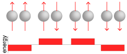 For the array as a whole, the energy is minimized if all the spins point the same way, either up or down. Each spin contributes a tiny magnetic moment. When the spins are parallel, all the moments add up and the system is fully magnetized.
If energy were the only consideration, the Ising model would always settle into a magnetized configuration, but there is a countervailing influence: Heat tends to randomize the spin directions. At infinite temperature, thermal fluctuations completely overwhelm the spins’ tendency to align, and all states are equally likely. Because the vast majority of those \(2^{10{,}000}\) configurations have nearly equal numbers of up and down spins, the magnetization is negligible. At zero temperature, nothing prevents the system from condensing into the fully magnetized state. The interval between these limits is a battleground where energy and entropy contend for supremacy. Clearly, there must be a transition of some kind. For Lenz and Ising in the 1920s, the crucial question was whether the transition comes at a sharply defined critical temperature, as it does in real ferromagnets. A more gradual progression from one regime to the other would signal the model’s failure to capture important aspects of ferromagnet physics.
In his doctoral dissertation Ising investigated the one-dimensional version of the model—a chain or ring of spins, each one holding hands with its two nearest neighbors. The result was a disappointment: He found no abrupt phase transition. And he speculated that the negative result would also hold in higher dimensions. The Ising model seemed to be dead on arrival.
It was revived a decade later by Rudolf Peierls, who gave suggestive evidence for a sharp transition in the two-dimensional lattice. Then in 1944 Lars Onsager “solved” the two-dimensional model, showing that the phase transition does exist. The phase diagram looks like this:
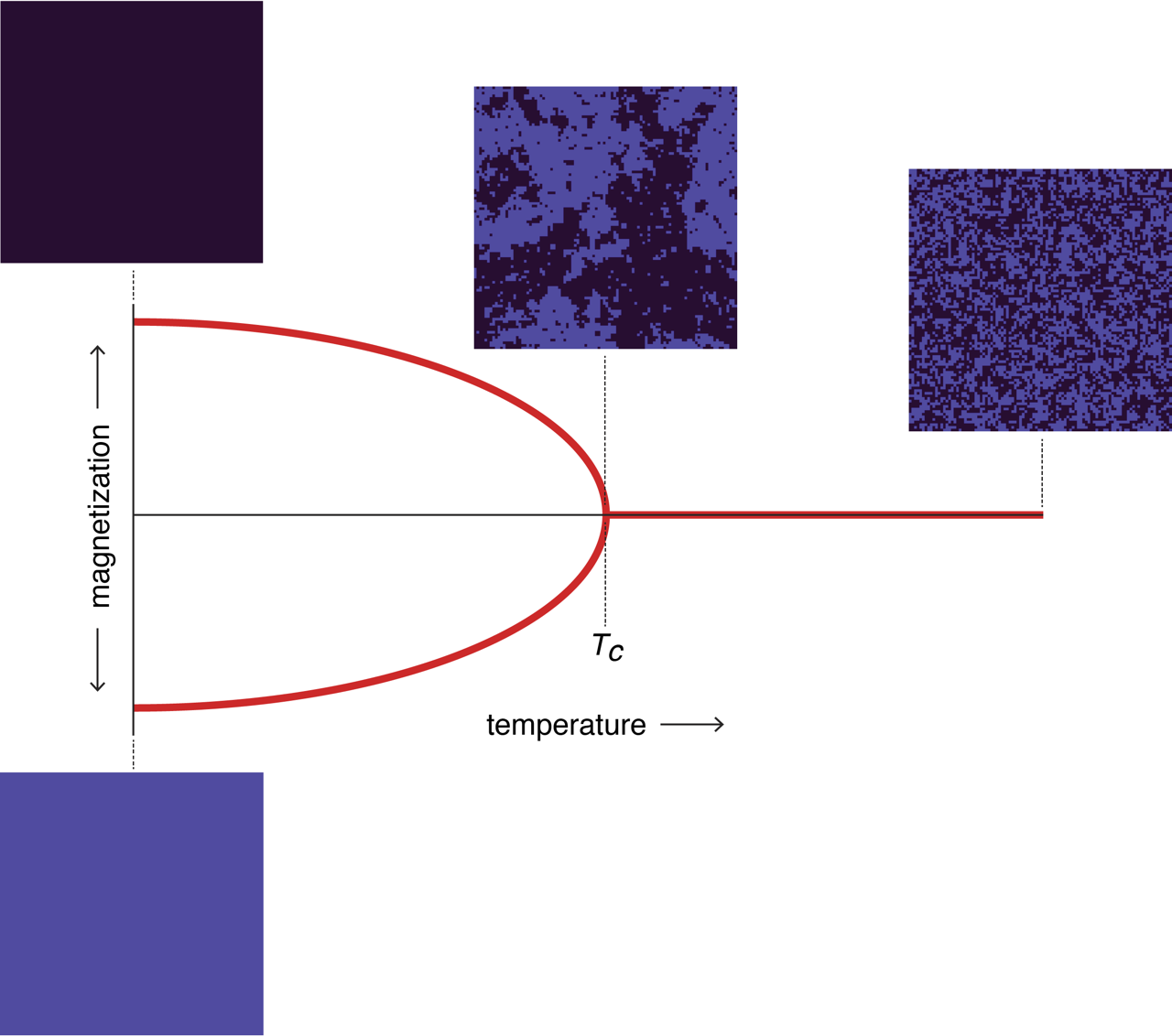
As the system cools, the salt-and-pepper chaos of infinite temperature evolves into a structure with larger blobs of color, but the up and down spins remain balanced on average (implying zero magnetization) down to the critical temperature \(T_C\). At that point there is a sudden bifurcation, and the system will follow one branch or the other to full magnetization at zero temperature.
If a model is classified as solved, is there anything more to say about it? In this case, I believe the answer is yes. The solution to the two-dimensional Ising model gives us a prescription for calculating the probability of seeing any given configuration at any given temperature. That’s a major accomplishment, and yet it leaves much of the model’s behavior unspecified. The solution defines the probability distribution at equilibrium—after the system has had time to settle into a statistically stable configuration. It doesn’t tell us anything about how the lattice of spins reaches that equilibrium when it starts from an arbitrary initial state, or how the system evolves when the temperature changes rapidly.
It’s not just the solution to the model that has a few vague spots. When you look at the finer details of how spins interact, the model itself leaves much to the imagination. When a spin reacts to the influence of its nearest neighbors, and those neighbors are also reacting to one another, does everything happen all at once? Suppose two antiparallel spins both decide to flip at the same time; they will be left in a configuration that is still antiparallel. It’s hard to see how they’ll escape repeating the same dance over and over, like people who meet head-on in a corridor and keep making mirror-image evasive maneuvers. This kind of standoff can be avoided if the spins act sequentially rather than simultaneously. But if they take turns, how do they decide who goes first?
Within the intellectual traditions of physics and mathematics, these questions can be dismissed as foolish or misguided. After all, when we look at the procession of the planets orbiting the sun, or at the colliding molecules in a gas, we don’t ask who takes the first step; the bodies are all in continuous and simultaneous motion. Newton gave us a tool, calculus, for understanding such situations. If you make the steps small enough, you don’t have to worry so much about the sequence of marching orders.
However, if you want to write a computer program simulating a ferromagnet (or simulating planetary motions, for that matter), questions of sequence and synchrony cannot be swept aside. With conventional computer hardware, “let everything happen at once” is not an option. The program must consider each spin, one at a time, survey the surrounding neighborhood, apply an update rule that’s based on both the state of the neighbors and the temperature, and then decide whether or not to flip. Thus the program must choose a sequence in which to visit the lattice sites, as well as a sequence in which to visit the neighbors of each site, and those choices can make a difference in the outcome of the simulation. So can other details of implementation. Do we look at all the sites, calculate their new spin states, and then update all those that need to be flipped? Or do we update each spin as we go along, so that spins later in the sequence will see an array already modified by earlier actions? The original definition of the Ising model is silent on such matters, but the programmer must make a commitment one way or another.
This is where Glauber dynamics enters the story. Glauber presented a version of the Ising model that’s somewhat more explicit about how spins interact with one another and with the “heat bath” that represents the influence of temperature. It’s a theory of Ising dynamics because he describes the spin system not just at equilibrium but also during transitional stages. I don’t know if Glauber was the first to offer an account of Ising dynamics, but the notion was certainly not commonplace in 1963.
There’s no evidence Glauber was thinking of his method as an algorithm suitable for computer implementation. The subject of simulation doesn’t come up in his 1963 paper, where his primary aim is to find analytic expressions for the distribution of up and down spins as a function of time. (He did this only for the one-dimensional model.) Nevertheless, Glauber dynamics offers an elegant approach to programming an interactive version of the Ising model. Assume we have a lattice of \(N\) spins. Each spin \(\sigma\) is indexed by its coordinates \(x, y\) and takes on one of the two values \(+1\) and \(-1\). Thus flipping a spin is a matter of multiplying \(\sigma\) by \(-1\). The algorithm for a updating the lattice looks like this:
Repeat \(N\) times:
- Choose a spin \(\sigma_{x, y}\) at random.
- Sum the values of the four neighboring spins, \(S = \sigma_{x+1, y} + \sigma_{x-1, y} + \sigma_{x, y+1} + \sigma_{x, y-1}\). The possible values of \(S\) are \(\{-4, -2, 0, +2, +4\}\).
- Calculate \(\Delta E = 2 \, \sigma_{x, y} \, S\), the change in interaction energy if \(\sigma_{x, y}\) were to flip.
- If \(\Delta E \lt 0\), set \(\sigma_{x, y} = -\sigma_{x, y}\).
- Otherwise, set \(\sigma_{x, y} = -\sigma_{x, y}\) with probability \(\exp(-\Delta E/T)\), where \(T\) is the temperature.
Display the updated lattice.
Step 4 says: If flipping a spin will reduce the overall energy of the system, flip it. Step 5 says: Even if flipping a spin raises the energy, go ahead and flip it in a randomly selected fraction of the cases. The probability of such spin flips is the Boltzmann factor \(\exp(-\Delta E/T)\). This quantity goes to \(0\) as the temperature \(T\) falls to \(0\), so that energetically unfavorable flips are unlikely in a cold lattice. The probability approaches \(1\) as \(T\) goes to infinity, which is why the model is such a seething mass of fluctuations at high temperature.
(If you’d like to take a look at real code rather than pseudocode—namely the JavaScript program running the simulation above—it’s on GitHub.)
Glauber dynamics belongs to a family of methods called Markov chain Monte Carlo algorithms (MCMC). The idea of Markov chains was an innovation in probability theory in the early years of the 20th century, extending classical probability to situations where the the next event depends on the current state of the system. Monte Carlo algorithms emerged at post-war Los Alamos, not long after Glauber left there to resume his undergraduate curriculum. He clearly kept up with the work of Stanislaw Ulam and other former colleagues in the Manhattan Project.
Within the MCMC family, the distinctive feature of Glauber dynamics is choosing spins at random. The obvious alternative is to march methodically through the lattice by columns and rows, examining every spin in turn. 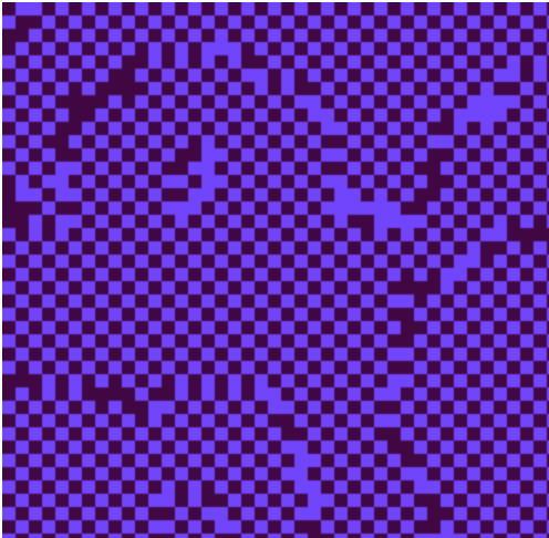 That procedure can certainly be made to work, but it requires care in implementation. At low temperature the Ising process is very nearly deterministic, since unfavorable flips are extremely rare. When you combine a deterministic flip rule with a deterministic path through the lattice, it’s easy to get trapped in recurrent patterns. For example, a subtle bug yields the same configuration of spins on every step, shifted left by a single lattice site, so that the pattern seems to slide across the screen. Another spectacular failure gives rise to a blinking checkerboard, where every spin is surrounded by four opposite spins and flips on every time step. Avoiding these errors requires much fussy attention to algorithmic details. (My personal experience is that the first attempt is never right.)
Choosing spins by throwing random darts at the lattice turns out to be less susceptible to clumsy mistakes. Yet, at first glance, the random procedure seems to have hazards of its own. In particular, choosing 10,000 spins at random from a lattice of 10,000 sites does not guarantee that every site will be visited once. On the contrary, a few sites will be sampled six or seven times, and you can expect that 3,679 sites (that’s \(1/e \times 10{,}000)\) will not be visited at all. Doesn’t that bias distort the outcome of the simulation? No, it doesn’t. After many iterations, all the sites will get equal attention.
The nasty bit in all Ising simulation algorithms is updating pairs of adjacent sites, where each spin is the neighbor of the other. Which one goes first, or do you try to handle them simultaneously? The column-and-row ordering maximizes exposure to this problem: Every spin is a member of such a pair. Other sequential algorithms—for example, visiting all the black squares of a checkerboard followed by all the white squares—avoid these confrontations altogether, never considering two adjacent spins in succession. Glauber dynamics is the Goldilocks solution. Pairs of adjacent spins do turn up as successive elements in the random sequence, but they are rare events. Decisions about how to handle them have no discernible influence on the outcome.
Years ago, I had several opportunities to meet Roy Glauber. Regrettably, I failed to take advantage of them. Glauber’s office at Harvard was in the Lyman Laboratory of Physics, a small isthmus building connecting two larger halls. In the 1970s I was a frequent visitor there, pestering people to write articles for Scientific American. It was fertile territory; for a few years, the magazine found more authors per square meter in Lyman Lab than anywhere else in the world. But I never knocked on Glauber’s door. Perhaps it’s just as well. I was not yet equipped to appreciate what he had to say.
Now I can let him have the last word. This is from the introduction to the paper that introduced Glauber dynamics:
If the mathematical problems of equilibrium statistical mechanics are great, they are at least relatively well-defined. The situation is quite otherwise in dealing with systems which undergo large-scale changes with time. The principles of nonequilibrium statistical mechanics remain in largest measure unformulated. While this lack persists, it may be useful to have in hand whatever precise statements can be made about the time-dependent hehavior of statistical systems, however simple they may be.
The Ising spin simulation model you discuss in this article is the basis of the combinatorial optimization method known as “simulated annealing”, which was introduced in a 1983 paper titled “Optimization by Simulated Annealing” by Scott Kirkpatrick et al. In particular, steps 3 through 5 of your program above constitute the inner loop of a typical SA program. An outer loop slowly lowers the “temperature” as the program runs, leading to a nearly optimal state as the temperature approaches zero.
Kirkpatrick’s paper mentions Ising and Nicholas Metropolis but does not mention Glauber.
That’s because the algorithm this blog post describes is NOT Glauber’s algorithm, but the Metropolis-Hastings algorithm instead. Glauber dynamics is something else (and is quite well described on Wikipedia).
This article was a great read! Plenty of simple explanations, and discussion of details I don’t usually see elsewhere. Thanks!
Also, I’m not sure if it was like this in the original source, but there’s a typo in the quote at the end:
“time-dependent hehavior of statistical systems”