My God, It’s Full of Dots!
by Brian Hayes
Published 27 September 2019
Please click or tap in the gray square below. It will fill with a jolly tableau of colored disks—first big blue ones, then somewhat smaller purple ones, and eventually lots of tiny red dots.
Sorry. My program and your browser are not getting along. None of the interactive elements of this page will work. Could you try a different browser? Current versions of Chrome, Firefox, and Safari seem to work.
The disks are scattered randomly, except that no disk is allowed to overlap another disk or extend beyond the boundary of the square. Once a disk has been placed, it never moves, so each later disk has to find a home somewhere in the nooks and crannies between the earlier arrivals. Can this go on forever?
The search for a vacant spot would seem to grow harder as the square gets more crowded, so you might expect the process to get stuck at some point, with no open site large enough to fit the next disk. On the other hand, because the disks get progressively smaller, later ones can squeeze into tighter quarters. In the specific filling protocol shown here, these two trends are in perfect balance. The process of adding disks, one after another, never seems to stall. Yet as the number of disks goes to infinity, they completely fill the box provided for them. There’s a place for every last dot, but there’s no blank space left over.
Or at least that’s the mathematical ideal. The computer program that fills the square above never attains this condition of perfect plenitude. It shuts down after placing just 5,000 disks, which cover about 94 percent of the square’s area. This early exit is a concession to the limits of computer precision and human patience, but we can still dream of how it would work in a world without such tiresome constraints.
This scheme for filling space with randomly placed objects is the invention of John Shier, a physicist who worked for many years in the semiconductor industry and who has also taught at Normandale Community College near Minneapolis. He explains the method and the mathematics behind it in a recent book, Fractalize That! A Visual Essay on Statistical Geometry. (For bibliographic details see the links and references at the end of this essay.) I learned of Shier’s work from my friend Barry Cipra.
Shier hints at the strangeness of these doings by imagining a set of 100 round tiles in graduated sizes, with a total area approaching one square meter. He would give the tiles to a craftsman with these instructions:
“Mark off an area of one square meter, either a circle or a square. Start with the largest tile, and attach it permanently anywhere you wish in the marked-off area. Continue to attach the tiles anywhere you wish, proceeding always from larger to smaller. There will always be a place for every tile regardless of how you choose to place them.” How many experienced tile setters would believe this?
Shier’s own creations go way beyond squares and circles filled with simple shapes such as disks.  He has shown that the algorithm also works with an assortment of more elaborate designs, including nonconvex figures and even objects composed of multiple disconnected pieces. We get snowflakes, nested rings, stars, butterflies, fish eating lesser fish, faces, letters of the alphabet, and visual salads bringing together multiple ingredients. Shier’s interest in these patterns is aesthetic as well as mathematical, and several of his works have appeared in art exhibits; one of them won a best-of-show award at the 2017 Joint Mathematics Meeting.
Shier and his colleagues have also shown that the algorithm can be made to work in three-dimensional space. The book’s cover is adorned with a jumble of randomly placed toruses filling the volume of a transparent cube. If you look closely, you’ll notice that some of the rings are linked; they cannot be disentangled without breaking at least one ring. (The 3D illustration was created by Paul Bourke, who has more examples online, including 3D-printed models.)
After reading Shier’s account of his adventures, and admiring the pictures, I had to try it for myself. The experiments I’m presenting in this essay have no high artistic ambitions. I stick with plain-vanilla circular disks in a square frame, all rendered with the same banal blue-to-red color scheme. My motive is merely to satisfy my curiosity—or perhaps to overcome my skepticism. When I first read the details of how these graphics are created, I couldn’t quite believe it would work. Writing my own programs and seeing them in action has helped persuade me. So has a proof by Christopher Ennis, which I’ll return to below.
Filling a region of the plane with disks is not in itself such a remarkable trick.  One well-known way of doing it goes by the name Apollonian circles. Start with three disks that are all tangent to one another, leaving a spiky three-pointed vacancy between them. Draw a new disk in the empty patch, tangent to all three of the original disks; this is the largest disk that can possibly fit in the space. Adding the new disk creates three smaller triangular voids, where you can draw three more triply tangent disks. There’s nothing to stop you from going on in this way indefinitely, approaching a limiting configuration where the entire area is filled.
There are randomized versions of the Apollonian model. For example, you might place zero-diameter seed disks at random unoccupied positions and then allow them to grow until they touch one (or more) of their neighbors. This process, too, is space-filling in the limit. And it can never fail: Because the disks are custom-fitted to the space available, you can never get stuck with a disk that can’t find a home.
Shier’s algorithm is different. You are given disks one at a time in a predetermined order, starting with the largest, then the second-largest, and so on. To place a disk in the square, you choose a point at random and test to see if the disk will fit at that location without bumping into its neighbors or poking beyond the boundaries of the square. If the tests fail, you pick another random point and try again. It’s not obvious that this haphazard search will always succeed—and indeed it works only if the successive disks get smaller according to a specific mathematical rule. But if you follow that rule, you can keep adding disks forever. Furthermore, as the number of disks goes to infinity, the fraction of the area covered approaches \(1\). It’s convenient to have a name for series of disks that meet these two criteria; I have taken to calling them fulfilling series.
In exploring these ideas computationally, it makes sense to start with the simplest case: disks that are all the same size. This version of the process clearly cannot be fulfilling. No matter how the disks are arranged, their aggregate area will eventually exceed that of any finite container. Click in the gray square below to start filling it with equal-size disks. The square box has area \(A_{\square} = 4\). The slider in the control panel determines the area of the individual disks \(A_k\), in a range from \(0.0001\) to \(1.0\).
Program 1: Fixed-Size Disks
Sorry, the program will not run in this browser.
If you play with this program for a while, you’ll find that the dots bloom quickly at first, but the process invariably slows down and eventually ends in a state labeled “Jammed,” indicating that the program has been unable The program gives up after trying 10 million random locations. to find a place where one more disk will fit. If you move the slider to the right, specifying larger disks, this impasse is reached very quickly, sometimes after placing just one or two disks. If you select very small disks, the program may churn away for five or ten minutes and fill the square with more than 20,000 disks before running out of options. Nevertheless, for any disk size greater than zero, a jammed outcome is inescapable.
The densest possible packing of equal-size disks places the centers on a triangular lattice with spacing equal to the disk diameter. The resulting density (for an infinite number of disks on an infinite plane) is \(\pi \sqrt{3}\, /\, 6 \approx 0.9069\), which means more than 90 percent of the area is covered. A random filling in a finite square is much looser. My first few trials all halted with a filling fraction fairly close to one-half, and so I wondered if that nice round number might be the expectation value of the probabilistic process. Further experiments suggested otherwise. Over a broad range of disk sizes, from \(0.0001\) up to about \(0.01\), the area covered varied from one run to the next, but the average was definitely above one-half—perhaps \(0.54\). After some rummaging through the voluminous literature on circle packing, I think I may have a clue to the exact expectation value: \(\pi / (3 + 2 \sqrt{2}) \approx 0.539012\). Where does that weird number come from? The answer has nothing to do with Shier’s algorithm, but I think it’s worth a digression.
 Consider an adversarial process: Alice is filling a unit square with \(n\) equal-size disks and wants to cover as much of the area as possible. Bob, who wants to minimize the area covered, gets to choose \(n\). If Bob chooses \(n = 1\), Alice can produce a single disk that just fits inside the square and covers about \(79\) percent of the space. Can Bob do better? Yes, if Bob specifies \(n = 2\), Alice’s best option is to squeeze the two disks into diagonally opposite corners of the square as shown in the diagram at right. These disks are bounded by right isosceles triangles, which makes it easy to calculate their radii as \(r = 1 / (2 + \sqrt{2}) \approx 0.2929\). Their combined area works out to that peculiar number \(\pi / (3 + 2 \sqrt{2}) \approx 0.54\).
If two disks are better than one (from Bob’s point of view), could three be better still? Or four, or some larger number? Apparently not. In 2010, Erik Demaine, Sándor Fekete and Robert Lang conjectured that the two-disk configuration shown above represents the worst case for any number of equal-size disks. In 2017 Fekete, Sebastian Morr, and Christian Scheffer proved this result.
Is it just a coincidence that the worst-case density for packing disks into a square also appears to be the expected density when equal-size disks are placed randomly until no more will fit? Wish I knew.
Let us return to the questions raised in Shier’s Fractalize That! If we want to fit infinitely many disks into a finite square, our only hope is to work with disks that get smaller and smaller as the process goes on. The disk areas must come from some sequence of ever-diminishing numbers. Among such sequences, the one that first comes to mind is \(\frac{1}{1}, \frac{1}{2}, \frac{1}{3}, \frac{1}{4}, \ldots\) These fractions have been known since antiquity as the harmonic numbers. (They are the wavelengths of the overtones of a plucked string.)
To see what happens when successive disks are sized according to the harmonic sequence, click in the square below.
Program 2: Disk Sizes from Harmonic Series
Sorry, the program will not run in this browser.
Again, the process halts when no open space is large enough to accommodate the next disk in the sequence. If you move the slider all the way to the right, you’ll see a sequence of disks with areas drawn from the start of the full harmonic sequence, \(\frac{1}{1} , \frac{1}{2}, \frac{1}{3}, \dots\); at this setting, you’ll seldom get beyond eight or nine disks. Moving the slider to the left omits the largest disks at the beginning of the sequence, leaving the infinite tail of smaller disks. For example, setting the slider to \(1/20\) skips all the disks from \(\frac{1}{1}\) through \(\frac{1}{19}\) and begins filling the square with disks of area \(\frac{1}{20}, \frac{1}{21}, \frac{1}{22}, \dots\) Such truncated series go on longer, but eventually they also end in a jammed configuration.
The slider goes no further than 1/50, but even if you omitted the first 500 disks, or the first 5 million, the result would be the same. This is a consequence of the most famous property of the harmonic numbers: Although the individual terms \(1/k\) dwindle away to zero as \(k\) goes to infinity, the sum of all the terms,
\[\sum_{k = 1}^{\infty}\frac{1}{k} = \frac{1}{1} + \frac{1}{2} + \frac{1}{3} + \cdots,\]
does not converge to a finite value. As long as you keep adding terms, the sum will keep growing, though ever more slowly. This curious fact was proved in the 14th century by the French bishop and scholar Nicole Oresme. The proof is simple but ingenious. Oresme pointed out that the harmonic sequence
\[\frac{1}{1} + \frac{1}{2} + \left(\frac{1}{3} + \frac{1}{4}\right) + \left(\frac{1}{5} + \frac{1}{6} + \frac{1}{7} + \frac{1}{8}\right) + \cdots\]
is greater than
\[\frac{1}{1} + \frac{1}{2} + \left(\frac{1}{4} + \frac{1}{4}\right) + \left(\frac{1}{8} + \frac{1}{8} + \frac{1}{8} + \frac{1}{8}\right) + \cdots\]
The latter series is equivalent to \(1 + \frac{1}{2} + \frac{1}{2} + \frac{1}{2} \cdots\), and so it is clearly divergent. Since the grouped terms of the harmonic series are even greater, they too must exceed any finite bound.
The divergence of the harmonic series implies that disks whose areas are generated by the series will eventually overflow any enclosing container. Dropping a finite prefix of the sequence, such as the first 50 disks, does not change this fact.
Let me note in passing that just as the filling fraction for fixed-size disks seems to converge to a specific constant, 0.5390, disks in harmonic series also seem to have a favored filling fraction, roughly 0.71. Can this be explained by some simple geometric argument? Again, I wish I knew.
Evidently we need to make the disks shrink faster than the harmonic numbers do. Here’s an idea: Square each element of the harmonic series, yielding this:
\[\sum_{k = 1}^{\infty}\frac{1}{k^2} = \frac{1}{1^2} + \frac{1}{2^2} + \frac{1}{3^2} + \cdots.\]
Click below (or press the Start button) to see how this one turns out, again in a square of area 4.
Program 3: Disk Sizes from Zeta(2)
Sorry, the program will not run in this browser.
At last we have a process that won’t get stuck in a situation where there’s no place to put another disk. It could run forever, but of course it doesn’t. It quits when the area of the next disk shrinks down to about a tenth of the size of a single pixel on a computer display. The stopped state is labeled “Exhausted” rather than “Jammed.”This is an algorithm that could truly run forever. And yet the result is still not quite what we were hoping for—it’s not fulfilling. The disks are scattered sparsely in the square, leaving vast open spaces unoccupied. The configuration reminds me of deep-sky images made by large telescopes.
Why does this outcome look so different from the others? Unlike the harmonic numbers, the infinite series \(1 + \frac{1}{4} + \frac{1}{9} + \frac{1}{16} + \cdots\) converges to a finite sum. In the 18th century the task of establishing this fact (and determining the exact sum) was known as the Basel Problem, after the hometown of the Bernoulli family, who put much effort into the problem but never solved it. The answer came in 1735 from Leonhard Euler (another native of Basel, though he was working in St. Petersburg), who showed that the sum is equal to \(\pi^2 / 6\). This works out to about \(1.645\); since the area of the square we want to fill is \(4\), even an infinite series of disks would cover only about \(41\) percent of the territory.
Given that the numbers \(\frac{1}{1^1}, \frac{1}{2^1}, \frac{1}{3^1}, \dots\) diminish too slowly, whereas \(\frac{1}{1^2}, \frac{1}{2^2}, \frac{1}{3^2}, \dots\) shrink too fast, it makes sense to try an exponent somewhere between \(1\) and \(2\) in the hope of finding a Goldilocks solution. The computation performed below in Program 4 is meant to facilitate the search for such a happy medium. Here the disk sizes are elements of the sequence \(\frac{1}{1^s}, \frac{1}{2^s}, \frac{1}{3^s}, \dots\), where the value of the exponent \(s\) is determined by the setting of the slider, with a range of \(1 \lt s \le 2\). We already know what happens at the extremes of this range. What is the behavior in the middle?
Program 4: Disk Sizes from Zeta(s)
Sorry, the program will not run in this browser.
If you try the default setting of \(s = 1.5\), you’ll find you are still in the regime where the disks dwindle away so quickly that the box never fills up; if you’re willing to wait long enough, the program will end in an exhausted state rather than a jammed one. Reducing the exponent to \(s = 1.25\) puts you on the other side of the balance point, where the disks remain too large and at some point one of them will not fit into any available space. By continuing to shuttle the slider back and forth, you could carry out a binary search, closing in, step by step, on the “just right” value of \(s\). This strategy can succeed, but it’s not quick. As you get closer to the critical value, the program will run longer and longer before halting. (After all, running forever is the behavior we’re seeking.) To save you some tedium, I offer a spoiler: the optimum setting is between 1.29 and 1.30.
At this point we have wandered into deeper mathematical waters. A rule of the form \(A_k = 1/k^s\) is called a power law, since each \(k\) is raised to the same power. And series of the form \(\sum 1/k^s\) are known as zeta functions, denoted \(\zeta(s)\). Zeta functions have quite a storied place in mathematics. The harmonic numbers correspond to \(\zeta(1) = \sum 1/k^1\), which does not converge. If \(\zeta(1)\) grows without limit whereas \(\zeta(2)\) converges, you might well wonder where the boundary lies between these two behaviors. As it happens, \(\zeta(1 + \epsilon)\) converges for any \(\epsilon \gt 0\).As mentioned above, Euler found that \(\zeta(2) = \pi^2 / 6\), and he went on to show that \(\zeta(s)\) also converges for all integer values of \(s\) greater than \(1\). Later, Pafnuty Chebyshev extended the domain of the function beyond the integers to all real numbers \(s\) greater than \(1\). And then Bernhard Riemann went further still: He devised a smoke-and-mirrors trick for defining the zeta function over the entire plane of complex numbers, with the single exception of \(s = 1\).
Today, Riemann’s version of the zeta function is the engine (or enigma!) driving a major mathematical industry. Shier’s use of this apparatus in making fractal art is far removed from that heavy-duty research enterprise—but no less fascinating. Think of it as the zeta function on vacation.
If a collection of disks are to fill a square exactly, their aggregate area must equal the area of the square. This is a necessary condition though not a sufficient one. In all the examples I’ve presented so far, the containing square has an area of 4, so what’s needed is to find a value of \(s\) that satisfies the equation:
\[\zeta(s) = \sum_{k = 1}^{\infty}\frac{1}{k^s} = 4\]
Except for isolated values of \(s\), Those isolated values are the negative integers and the even positive integers.there is no known method for solving this equation exactly. But numerical approximation works well enough for a computer program that draws pictures. The binary search described above is a crude and cumbersome version of this numerical method. SageMath presumably does something more sophisticated. When I ask it to find a root of the equation \(zeta(s) = 4\), it returns the result \(1.2939615055572438\).
Having this result in hand solves one part of the square-filling problem. It tells us how to construct an infinite set of disks whose total area is just enough to cover a square of area \(4\), with adequate precision for graphical purposes. We assign each disk \(k\) (starting at \(k = 1\)) an area of \(1/k^{1.2939615}.\) This sequence begins 1.000, 0.408, 0.241, 0.166, 0.125, 0.098,…

In the graph above, the maroon curve with \(s = 1.29396\) converges to a sum very close to 4. Admittedly, the rate of convergence is not quick. More than 3 million terms are needed to get within 1 percent of the target.
Our off-label use of the zeta function defines an infinite sequence of disks whose aggregate area is equal to \(4\). The disks in this unique collection will exactly fill our square box (assuming they can be properly arranged). It’s satisfying to have a way of reliably achieving this result, after our various earlier failures. On the other hand, there’s something irksome about that number \(4\) appearing in the equation. It’s so arbitrary! I don’t dispute that \(4\) is a perfectly fine and foursquare number, but there are many other sizes of squares we might want to fill with dots. Why give all our attention to the \(2 \times 2\) variety?
This is all my fault. When I set out to write some square-filling programs, I knew I couldn’t use the unit square—which seems like the obvious default choice—because of the awkward fact that \(\zeta(s) = 1\) has no finite solution. The unit square is also troublesome in the case of the harmonic numbers; the first disk, with area \(A_1 = 1\), is too large to fit. So I picked the next squared integer for the box size in those first programs. Having made my choice, I stuck with it, but now I feel hemmed in by that decision made with too little forethought.
We have all the tools we need to fill squares of other sizes (as long as the size is greater than \(1\)). Given a square of area \(A_{\square}\), we just solve for \(s\) in \(\zeta(s) = A_{\square}\). A square of area 8 can be covered by disks sized according to the rule \(A_k = 1/k^s\) with \(s = \zeta(8) \approx 1.1349\). For \(A_{\square} = 100\), the corresponding value of \(s\) is \(\zeta(100) \approx 1.0101\). For any \(A_{\square} \gt 1\) there is an \(s\) that yields a fulfilling set of disks, and vice versa for any \(s \gt 1\).
This relation between the exponent \(s\) and the box area \(A_{\square}\) suggests a neat way to evade the whole bother of choosing a specific container size. We can just scale the disks to fit the box, or else scale the box to accommodate the disks. Shier adopts the former method. Each disk in the infinite set is assigned an area of
\[A_k = \frac{A_{\square}}{\zeta(s)} \frac{1}{k^s},\]
where the first factor is a scaling constant that adjusts the disk sizes to fit the container. In my first experiments with these programs I followed the same approach. Later, however, when I began writing this essay, it seemed easier to think about the scaling—and explain it—if I transformed the size of the box rather than the sizes of the disks. In this scheme, the area of disk \(k\) is simply \(1 / k^s\), and the area of the container is \(A_{\square} = \zeta(s)\). (The two scaling procedures are mathematically equivalent; it’s only the ratio of disk size to container size that matters.)
Program 5 offers an opportunity to play with such scaled zeta functions. I’m not actually changing the physical size of the box—the number of pixels it occupies on-screen remains the same. I’m scaling the units of measure.No matter where you move the \(s\) slider, the area of the square container will adjust to match the total area of the infinite set of disks. As the ratio of disk size to container size shifts, so does the overall texture or appearance of the pattern. At a setting of \(s = 1.35\), the largest disk fills almost a third of the square; at \(s = 1.08\), the first disk occupies only about \(8\) percent of box area. At those lower settings it takes a very long time to reach a high filling percentage, but if you have true faith in mathematical certainties, your patience will be rewarded.
Program 5: Disk Sizes from Scaled Zeta(s)
Sorry, the program will not run in this browser.
At the other end of the scale, if you push the value of \(s\) up beyond about \(1.40\), you’ll discover something else: The program more often than not halts after placing just a few disks. At \(s = 1.50\) or higher, it seldom gets beyond the first disk. This failure is similar to what we saw with the harmonic numbers, but more interesting. In the case of the harmonic numbers, the total area of the disks is unbounded, making an overflow inevitable. With this new scaled version of the zeta function, the total area of the disks is always equal to that of the enclosing square. In principle, all the disks could all be made to fit, if you could find the right arrangement. I’ll return below to the question of why that doesn’t happen.
In Fractalize That! Shier introduces another device for taming space-filling sets. He not only scales the object sizes so that their total area matches the space available; he also adopts a variant zeta function that has two adjustable parameters rather than just one:
A note on notation: Shier writes the Hurwitz zeta function as \(\zeta(c, N)\), whereas most of the mathematical literature seems to favor \(\zeta(s, a)\). I’m going with the majority.\[\zeta(s, a) = \sum_{k=0}^{\infty} \frac{1}{(a + k)^s}\]
This is the Hurwitz zeta function, named for the German mathematician Adolf Hurwitz (1859–1919). Before looking into the details of the function, let’s play with the program and see what happens. Try a few settings of the \(s\) and \(a\) controls:
Program 6: Disk Sizes from Scaled Hurwitz Zeta Function
Sorry, the program will not run in this browser.
Different combinations of \(s\) and \(a\) produce populations of disks with different size distributions. The separate contributions of the two parameters are not always easy to disentangle, but in general decreasing \(s\) or increasing \(a\) leads to a pattern dominated by smaller disks. Here are snapshots of four outcomes:

Within the parameter range shown in these four panels, the filling process always continues to exhaustion, but at higher values of \(s\) it can jam, just as it does with the scaled Riemann zeta function.
Adolf Hurwitz in the 1880s. Photo from Wikipedia. Until I began this project, I knew nothing of Adolf Hurwitz or his work, although he is hardly an obscure figure in the history of mathematics. He earned his Ph.D. under Felix Klein and also studied with Karl Weierstrass, Ernst Eduard Kummer, and Leopold Kronecker—key figures in the founding of modern analysis and number theory. Among his own pupils (and close friends) were David Hilbert and Hermann Minkowski. Albert Einstein was another of his students, although apparently he seldom went to class.
Hurwitz wrote just one paper on the zeta function. It was published in 1882, when he was still quite young and just beginning his first academic appointment, at the University of Göttingen. (The paper is available from the Göttinger Digitalisierungszentrum; see pp. 86–101.)
Hurwitz modified the Riemann zeta function in two ways. First, the constant \(a\) is added to each term, turning \(1/k^s\) into \(1/(a + k)^s\). Second, the summation begins with \(k = 0\) rather than \(k = 1\). By letting \(a\) take on any value in the range \(0 \lt a \le 1\) we gain access to a continuum of zeta functions. The elements of the series are no longer just reciprocals of integers but reciprocals of real numbers. Suppose \(a = \frac{1}{3}\). Then \(\zeta(s, a)\) becomes:
\[\frac{1}{\left(\frac{1}{3} + 0\right)^s} + \frac{1}{\left(\frac{1}{3} + 1\right)^s} + \frac{1}{\left(\frac{1}{3} + 2\right)^s} + \cdots\ = \left(\frac{3}{1}\right)^s + \left(\frac{3}{4}\right)^s + \left(\frac{3}{7}\right)^s + \cdots\]
 The Riemann zeta function and the Hurwitz zeta function differ substantially only for small values of \(k\) or large values of \(a\). When \(k\) is large, adding a small \(a\) to it makes little difference in the value of the function. Thus as \(k\) grows toward infinity, the two functions are asymptotically equal, as suggested in the graph at right. When the Hurwitz function is put to work packing disks into a square, a rule with \(a > 1\) causes the first several disks to be smaller than they would be with the Riemann rule. A value of \(a\) between \(0\) and \(1\) enlarges the early disks. In either case, the later disks in the sequence are hardly affected at all.
If \(a\) is a positive integer, the interpretation of \(\zeta(s, a)\) is even simpler. The case \(a = 1\) corresponds to the Riemann zeta sum. When \(a\) is a larger integer, the effect is to omit the first \(a - 1\) entries, leaving only the tail of the series. For example,
\[\zeta(s, 5) = \frac{1}{5^s} + \frac{1}{6^s} + \frac{1}{7^s} + \cdots.\]
In his fractal artworks, Shier chooses various values of \(a\) as a way of controlling the size distribution of the placed objects, and thereby fine-tuning the appearance of the patterns. Having this adjustment knob available is very convenient, but in the interests of simplicity, I am going to revert to the Riemann function in the rest of this essay.
Before going on, however, I also have to confess that I don’t really understand the place of the Hurwitz zeta function in modern mathematical research, or what Hurwitz himself had in mind when he formulated it. Zeta functions have been an indispensable tool in the long struggle to understand how the prime numbers are sprinkled among the integers. The connection between these two realms was made by Euler, with his remarkable equation linking a sum of powers of integers with a product of powers of primes:
Euler’s other famous equation, \(e^{i\pi} + 1 = 0\), has a bigger fan club, but this is the one that revs my motor.\[\sum_{k = 1}^{\infty} \frac{1}{k^s} = \prod_{p \text{ prime}} \frac{1}{1 - \frac{1}{p^s}}.\]
Riemann went further, showing that everything we might want to know about the distribution of primes is encoded in the undulations of the zeta function over the complex plane. Indeed, if we could simply pin down all the complex values of \(s\) for which \(\zeta(s) = 0\), we would have a master key to the primes. Hurwitz, in his 1882 paper, was clearly hoping to make some progress toward this goal, but I have not been able to figure out how his work fits into the larger story. The Hurwitz zeta function gets almost no attention in standard histories and reference works (in contrast to the Riemann version, which is everywhere). Wikipedia notes: “At rational arguments the Hurwitz zeta function may be expressed as a linear combination of Dirichlet L-functions and vice versa”—which sounds interesting, but I don’t know if it’s useful or important. A recent article by Nicola Oswald and Jörn Steuding puts Hurwitz’s work in historical context, but it does not answer these questions—at least not in a way I’m able to understand.
But again I digress. Back to dots in boxes.
If a set of circular disks and a square container have the same total area, can you always arrange the disks so that they completely fill the square without overflowing? Certainly not! Suppose the set consists of a single disk with area equal to that of the square; the disk’s diameter is greater than the side length of the square, so it will bulge through the sides while leaving the corners unfilled. A set of two disks won’t work either, no matter how you apportion the area between them. Indeed, when you are putting round pegs in a square hole, no finite set of disks can ever fill all the crevices.
Only an infinite set—a set with no smallest disk—can possibly fill the square completely. But even with an endless supply of ever-smaller disks, it seems like quite a delicate task to find just the right arrangement, so that every gap is filled and every disk has a place to call home. It’s all the more remarkable, then, that simply plunking down the disks at random locations seems to produce exactly the desired result. This behavior is what intrigued and troubled me when I first saw Shier’s pictures and read about his method for generating them. If a random arrangement works, it’s only a small step to the proposition that any arrangement works. Could that possibly be true?
Computational experiments offer strong hints on this point, but they can never be conclusive. What we need is a proof. Ennis’s proof was published in Math Horizons, a publication of the Mathematical Association of America, which keeps it behind a paywall. If you have no library access and won’t pay the $50 ransom, I can recommend a video of Ennis explaining his proof in a talk at St. Olaf College.And so I turn to the work of Christopher Ennis, a mathematician at Normandale Community College, who met Shier when they were both teaching there.
As a warm-up exercise, Ennis proves a one-dimensional version of the area-filling conjecture, where the geometry is simpler and some of the constraints are easier to satisfy. In one dimension a disk is merely a line segment; its area is its length, and its radius is half that length. As in the two-dimensional model, disks are placed in descending order of size at random positions, with the usual proviso that no disk can overlap another disk or extend beyond the end points of the containing interval. In Program 7 you can play with this scheme.
Program 7: One-Dimensional Disks
Sorry, the program will not run in this browser.
I have given the line segment some vertical thickness to make it visible. The resulting pattern of stripes may look like a supermarket barcode or an atomic spectrum, but please imagine it as one-dimensional.
If you adjust the slider in this program, you’ll notice a difference from the two-dimensional system. In 2D, the algorithm is fulfilling only if the exponent \(s\) is less than a critical value, somewhere in the neighborhood of 1.4. In one dimension, the process continues without impediment for all values of \(s\) throughout the range \(1 \lt s \lt 2\). Try as you might, you won’t find a setting that produces a jammed state. (In practice, the program halts after placing no more than 10,000 disks, but the reason is exhaustion rather than jamming.)
Ennis titles his Math Horizons article “(Always) room for one more.” He proves this assertion by keeping track of the set of points where the center of a new disk can legally be placed, and showing the set is never empty. Suppose \(n - 1\) disks have already been randomly scattered in the container. The next disk to be placed, disk \(n\), will have an area (or length) of \(A_n = 1 / n^s\). Since the geometry is one-dimensional, the corresponding disk radius is simply \(r_n = A_n / 2\). The center of this new disk cannot lie any closer than \(r_n\) to the perimeter of another disk. It must also be at a distance of at least \(r_n\) from the boundary of the containing segment. We can visualize these constraints by adding bumpers, or buffers, of thickness \(r_n\) to the outside of each existing disk and to the inner edges of the containing segment. A few stages of the process are illustrated below.

Placed disks are blue, the excluded buffer areas are orange, and open areas—the set of all points where the center of the next disk could be placed—are black. In the top line, before any disks have been placed, the entire containing segment is open except for the two buffers at the ends. Each of these buffers has a length equal to \(r_1\), the radius of the first disk to be placed; the center of that disk cannot lie in the orange regions because the disk would then overhang the end of the containing segment. After the first disk has been placed (second line), the extent of the open area is reduced by the area of the disk itself and its appended buffers. On the other hand, all of the buffers have also shrunk; each buffer is now equal to the radius of disk \(2\), which is smaller than disk \(1\). The pattern continues as subsequent disks are added. Note that although the blue disks cannot overlap, the orange buffers can.
For another view of how this process evolves, click on the Next button in Program 8. Each click inserts one more disk into the array and adjusts the buffer and open areas accordingly.
Program 8: One-Dimensional with Buffers
Sorry, the program will not run in this browser.
Because the blue disks are never allowed to overlap, the total blue area must increase monotonically as disks are added. It follows that the orange and black areas, taken together, must steadily decrease. But there’s nothing steady about the process when you keep an eye on the separate area measures for the orange and black regions. Changes in the amount of buffer overlap cause erratic, seesawing tradeoffs between the two subtotals. If you keep clicking the Next button (especially with \(s\) set to a high value), you may see the black area falling below \(1\) percent. Can we be sure it will never vanish entirely, leaving no opening at all for the next disk?
Ennis answers this question through worst-case analysis. He considers only configurations in which no buffers overlap, thereby squeezing the black area to its smallest possible extent. If the black area is always positive under these conditions, it cannot be smaller when buffer overlaps are allowed.
The basic idea of the proofI have altered some of the notation and certain details of presentation to conform with choices I made elsewhere in this exposition. is to start with \(n - 1\) buffered disks already in place, arranged so that none of the orange buffer areas intersect. The total area of the blue disks is \(\sum_{k=1}^{k=n-1} 1/k^s\). Each buffer zone has a width equal to \(r_{n}\), the radius of the next disk to be added to the tableau; since each disk has two buffers, the total area of the orange buffers is \(2(n-1)r_{n}\). The black area is whatever’s left over. In other words,
\[A_{\square} = \zeta(s), \quad A_{\color{blue}{\mathrm{blue}}} = \sum_{k=1}^{k = n - 1} \frac{1}{k^s}, \quad A_{\color{orange}{\mathrm{orange}}} = 2(n-1)r_{n}.\]
Then we need to prove that
\[A_{\square} - (A_{\color{blue}{\mathrm{blue}}} + A_{\color{orange}{\mathrm{orange}}}) \gt 0.\]
A direct proof of this statement would require an exact, closed-form expression for \(\zeta(s)\), which we already know is problematic. Ennis evades this difficulty by turning to calculus. He needs to evaluate the remaining tail of the zeta series, \(\sum_{k = n}^\infty 1/k^s\), but this discrete sum is intractable. On the other hand, by shifting from a sum to an integral, the problem becomes an exercise in undergraduate calculus. Exchanging the discrete variable \(k\) for a continuous variable \(x\), we want to find the area under the curve \(1/x^s\) in the interval from \(n\) to infinity; this will provide a lower bound on the corresponding discrete sum. Evaluating the integral yields:
\[\int_{x = n}^{\infty} \frac{1}{x^{s}} d x = \frac{1}{(s-1) n^{s-1}}.\]
Some further manipulation reveals that the area of the black regions is never smaller than
\[\frac{2 - s}{(s - 1)n^{s - 1}}.\]
If \(s\) lies strictly between \(1\) and \(2\), this expression must be greater than zero, since both the numerator and the denominator will be positive. Thus for all \(n\) there is at least one black point where the center of a new disk can be placed.
Ennis’s proof is a stronger one than I expected. When I first learned there was a proof, I guessed that it would take a probabilistic approach, showing that although a jammed configuration may exist, it has probability zero of turning up in a random placement of the disks. Instead, Ennis shows that no such arrangement exists at all. Even if you replaced the randomized algorithm with an adversarial one that tries its best to block every disk, the process would still run to fulfillment.
The proof for a two-dimensional system follows the same basic line of argument, but it gets more complicated for geometric reasons. In one dimension, as the successive disk areas get smaller, the disk radii diminish in simple proportion: \(r_k = A_k / 2\). In two dimensions, disk radius falls off only as the square root of the disk area: \(r_k = \sqrt{A_k / \pi}\). As a result, the buffer zone surrounding a disk excludes neighbors at a greater distance in two dimensions than it would in one dimension. There is still a range of \(s\) values where the process is provably unstoppable, but it does not extend across the full interval from \(s \gt 1\) to \(s \lt 2\).
Program 9, running in the panel below, is one I find very helpful in gaining intuition into the behavior of Shier’s algorithm. As in the one-dimensional model of Program 8, each press of the Next button adds a single disk to the containing square, and shows the forbidden buffer zones surrounding the disks.
Program 9: Two-Dimensional Disks with Buffers
Sorry, the program will not run in this browser.
Move the \(s\) slider to a position somewhere near 1.40. In the control panel for this program, the registers showing fill percentages for blue, orange, and black areas are not entirely trustworthy. In the one-dimensional case, it’s easy to calculate the areas to high precision. That’s much harder in two dimensions, where the overlapping regions of buffers can have complex shapes. I have resorted to counting pixels, a procedure that has limited resolution and is subject to errors caused by fuzzy boundaries.At this setting, there’s a fair chance (maybe 10 or 20 percent) that the very first disk and its orange buffer zone will entirely cover the open black region, creating a jammed state. On other runs you might get as far as two or three or 10 disks before you get stuck. If you make it beyond that point, however, you are likely to continue unimpeded for as long as you have the patience to keep pressing Next. Shier describes this phenomenon as “infant mortality”: If the placement process survives the high-risk early period, it is all but immortal.
There’s a certain whack-a-mole dynamic to the behavior of this system. Maybe the first disk covers all but one small corner of the black zone. It looks like the next disk will completely obliterate that open area. And so it does—but at the same time the shrinking of the orange buffer rings opens up another wedge of black elsewhere. The third disk blots out that spot, but again the narrowing of the buffers allows a black patch to peek out from still another corner. Later on, when there are dozens of disks, there are also dozens of tiny black spots where there’s room for another disk. You can often guess which of the openings will be filled next, because the random search process is likely to land in the largest of them. Again, however, as these biggest targets are buried, many smaller ones are born.
Ennis’s two-dimensional proof addresses the case of circular disks inside a circular boundary, rather than a square one. (The higher symmetry and the absence of corners streamlines certain calculations.) The proof strategy, again, is to show that after \(n - 1\) disks have been placed, there is still room for the \(n\)th disk, for any value of \(n \ge 1\). The argument follows the same logic as in one dimension, relying on an integral to provide a lower bound for the sum of a zeta series. But because of the \(\pi r^2\) area relation, the calculation now includes quadratic as well as linear terms. As a result, the proof covers only a part of the range of \(s\) values. The black area is provably nonempty if \(s\) is greater than \(1\) but less than roughly \(1.1\); outside that interval, the proof has nothing to say.
As mentioned above, Ennis’s proof applies only to circular disks in a circular enclosure. Nevertheless, in what follows I am going to assume the same ideas carry over to disks in a square frame, although the location of the boundary will doubtless be somewhat different. I have recently learned that Ennis has written a further paper on the subject, expected to be published in the American Mathematical Monthly. Perhaps he addresses this question there.
With Program 9, we can explore the entire spectrum of behavior for packing disks into a square. The possibilities are summarized in the candybar graph below.

- The leftmost band, in darker green, is the interval for which Ennis’s proof might hold. The question mark at the upper boundary line signifies that we don’t really know where it lies.
- In the lighter green region no proof is known, but in Shier’s extensive experiments the system never jams there.
- The transition zone sees the probability of jamming rise from \(0\) to \(1\) as \(s\) goes from about \(1.3\) to about \(1.5\).
- Beyond \(s \approx 1.5\), experiments suggest that the system always halts in a jammed configuration.
- At \(s \approx 1.6\) we enter a regime where the buffer zone surrounding the first disk invariably blocks the entire black region, leaving nowhere to place a second disk. Thus we have a simple proof that the system always jams.
- Still another barrier arises at \(s \approx 2.7\). Beyond this point, not even one disk will fit. The diameter of a disk with area \(1\) is greater than the side length of the enclosing square.
Can we pin down the exact locations of the various threshold points in the diagram above? This problem is tractable in those situations where the placement of the very first disk determines the outcome.  At high values of \(s\) (and thus low values of \(\zeta(s)\), the first disk can obliterate the black zone and thereby preclude placement of a second disk. What is the lowest value of \(s\) for which this can happen? As in the image at right, the disk must lie at the center of the square box, and the orange buffer zone surrounding it must extend just far enough out to cover the corners of the inner black square, which defines the locus of all points that could accommodate the center of the second disk. Finding the value of \(s\) that satisfies this condition is a messy but straightforward bit of geometry and algebra. With the help of SageMath I get the answer \(s = 1.282915\). This value—let’s call it \(\overline{s}\)—is an upper bound on the “never jammed” region. Above this limit there is always a nonzero probability that the filling process will end after placing a single disk.
The value of \(\overline{s}\) lies quite close to the experimentally observed boundary between the never-jammed range and the transition zone, where jamming first appears. Is it possible that \(\overline{s}\) actually marks the edge of the transition zone—that below this value of \(s\) the program can never fail? To prove that conjecture, you would have to show that when the first disk is successfully placed, the process never stalls on a subsequent disk. That’s certainly not true in higher ranges of \(s\). Yet the empirical evidence near the threshold is suggestive. In my experiments I have yet to see a jammed outcome at \(s \lt \overline{s}\), not even in a million trials just below the threshold, at \(s = 0.999 \overline{s}\). In contrast, at \(s = 1.001 \overline{s}\), a million trials produced 53 jammed results—all of them occuring immediately after the first disk was placed.
 The same kind of analysis leads to a lower bound on the region where every run ends after the first disk (medium pink in the diagram above). In this case the critical situation puts the first disk as close as possible to a corner of the square frame, rather than in the middle. If the disk and its orange penumbra are large enough to block the second disk in this extreme configuration, then they will also block it in any other position. Putting a number on this bound again requires some fiddly equation wrangling; the answer I get is \(\underline{s} = 1.593782\). No process with higher \(s\) can possibly live forever, since it will die with the second disk. In analogy with the lower-bound conjecture, one might propose that the probability of being jammed remains below \(1\) until \(s\) reaches \(\underline{s}\). If both conjectures were true, the transition region would extend from \(\overline{s}\) to \(\underline{s}\).
 The final landmark, way out at \(s \approx 2.7\), marks the point where the first disk threatens to burst the bounds of the enclosing square. In this case the game is over before it begins. In program 9, if you push the slider far to the right, you’ll find that the black square in the middle of the orange field shrinks away and eventually winks out of existence. This extinction event comes when the diameter of the disk equals the side length of the square. Given a disk of area \(1\), and thus radius \(1/\sqrt{\pi}\), we want to find the value of \(s\) that satisfies the equation
\[\frac{2}{\sqrt{\pi}} = \sqrt{\zeta(s)}.\]
Experiments with Program 9 show that the value is just a tad more than 2.7. That’s an interesting numerical neighborhood, no? A famous number lives nearby. Do you suppose?
Another intriguing set of questions concerns the phenomenon that Shier calls infant mortality. If you scroll back up to Program 5 and set the slider to \(s = 1.45\), you’ll find that roughly half the trials jam. The vast majority of these failures come early in the process, after no more than a dozen disks have been placed. At \(s = 1.50\) death at an early age is even more common; three-fourths of all the trials end with the very first disk. On the other hand, if a sequence of disks does manage to dodge all the hazards of early childhood, it may well live on for a very long time—perhaps forever.
Should we be surprised by this behavior? I am. As Shier points out, the patterns formed by our graduated disks are fractals, and one of their characteristic properties is self-similarity, or scale invariance. If you had a fully populated square—one filled with infinitely many disks—you could zoom in on any region to any magnification, and the arrangement of disks would look the same as it does in the full-size square. By “look the same” I don’t mean the disks would be in the same positions, but they would have the same size distribution and the same average number of neighbors at the same distances. This is a statistical concept of identity. And since the pattern looks the same and has the same statistics, you would think that the challenge of finding a place for a new disk would also be the same at any scale. Slipping in a tiny disk late in the filling operation would be no different from plopping down a large disk early on. The probability of jamming ought to be constant from start to finish.
But there’s a rejoinder to this argument: Scale invariance is broken by the presence of the enclosing square. The largest disks are strongly constrained by the boundaries, whereas most of the smaller disks are nowhere near the edges and are little influenced by them. The experimental data offer some support for this view. The graph below summarizes the outcomes of \(20{,}000\) trials at \(s = 1.50\). The red bars show the absolute numbers of trials ending after placing \(n\) disks, for each \(n\) from \(0\) through \(35\). The blue lollipops indicate the proportion of trials reaching disk \(n\) that halted after placing disk \(n\). This ratio can be interpreted (if you’re a frequentist!) as the probability of stopping at \(n\).

It certainly looks like there’s something odd happening on the left side of this graph. More than three fourths of the trials end after a single disk, but none at all jam at the second or third disks, and very few (a total of \(23\)) at disks \(4\) and \(5\). Then, suddenly, \(1{,}400\) more fall by the wayside at disk \(6\), and serious attrition continues through disk \(11\).
Geometry can explain some of this weirdness. It has to do with the squareness of the container; other shapes would produce different results.
At \(s = 1.50\) we are between \(\overline{s}\) and \(\underline{s}\), in a regime where the first disk is large enough to block off the entire black zone but not so large that it must do so. This is enough to explain the tall red bar at \(n = 1\): When you place the first disk randomly, roughly \(75\) percent of the time it will block the entire black region, ending the parade of disks. If the first disk doesn’t foreclose all further action, it must be tucked into one of the four corners of the square, leaving enough room for a second disk in the diagonally opposite corner. The sequence of images below (made with Program 9) tells the rest of the story.

The placement of the second disk blocks off the open area in that corner, but the narrowing of the orange buffers also creates two tiny openings in the cross-diagonal corners. The third and fourth disks occupy these positions, and simultaneously allow the black background to peek through in two other spots. Finally the fifth and sixth disks close off the last black pixels, and the system jams.
This stereotyped sequence of disk placements accounts for the near absence of mortality at ages \(n = 2\) through \(n = 5\), and the sudden upsurge at age \(6\). The elevated levels at \(n = 7\) through \(11\) are part of the same pattern; depending on the exact positioning of the disks, it may take a few more to expunge the last remnants of black background.
At still higher values of \(n\)—for the small subset of trials that get there—the system seems to shift to a different mode of behavior. Although numerical noise makes it hard to draw firm conclusions, it doesn’t appear that any of the \(n\) values beyond \(n = 12\) are more likely jamming points than others. Indeed, the data are consistent with the idea that the probability of jamming remains constant as each additional disk is added to the array, just as scale invariance would suggest.
A much larger data set would be needed to test this conjecture, and collecting such data is painfully slow. Furthermore, when it comes to rare events, I don’t have much trust in the empirical data. During one series of experiments, I noticed a program run that stalled after \(290\) disks—unusually late. The 290-disk configuration, produced at \(s = 1.47\), is shown at left below.
This pattern, compared with those produced at lower values of \(s\), has a strongly Apollonian texture. Many of the disks are nestled tightly among their neighbors, and they form the recursive triangular motifs characteristic of Apollonian circles.
I wondered if it was truly jammed. My program gives up on finding a place for a disk after \(10^7\) random attempts. Perhaps if I had simply persisted, it would have gone on. So I reset the limit on random attempts to \(10^9\), and sat back to wait. After some minutes the program discovered a place where disk \(291\) would fit, and then another for disk \(292\), and kept going as far as 300 disks. The program had an afterlife! Could I revive it again? Upping the limit to \(10^{10}\) allowed another \(14\) disks to squueze in. The final configuration is shown at right above (with the original \(290\) disks faded, in order to make the \(24\) posthumous additions more conspicuous).
Is it really finished now, or is there still room for one more? I have no reliable way to answer that question. Checking \(10\) billion random locations sounds like a lot, but it is still a very sparse sampling of the space inside the square box. Using 64-bit floating-point numbers to define the coordinate system allows for more than \(10^{30}\) distinguishable points. And to settle the question mathematically, we would need unbounded precision.
We know from Ennis’s proof that at values of \(s\) not too far above \(1.0\), the filling process can always go on forever. And we know that beyond \(s \approx 1.6\), every attempt to fill the square is doomed. There must be some kind of transition between these two conditions, but the details are murky. The experimental evidence gathered so far suggests a smooth transition along a sigmoid curve, with the probability of jamming gradually increasing from \(0\) to \(1\). As far as I can tell, however, nothing we know for certain rules out a single hard threshold, below which all disk sequences are immortal and above which all of them die. Thus the phase diagram would be reduced to this simple form:

The softer transition observed in computational experiments would be an artifact of our inability to perform infinite random searches or place infinite sequences of disks.
Here’s a different approach to understanding the random dots-in-a-box phenomenon. It calls for a mental reversal of figure and ground. Instead of placing disks on a square surface, we drill holes in a square metal plate. And the focus of attention is not the array of disks or holes but rather the spaces between them. Shier has a name for the perforated plate: the gasket.
Program 10 allows you to observe a gasket as it evolves from a solid black square to a delicate lace doily with less than 1 percent of its original substance.
Program 10: The Gasket
Sorry, the program will not run in this browser.
The gasket is quite a remarkable object. When the number of holes becomes infinite, the gasket must disappear entirely; its area falls to zero. Up until that very moment, however, it retains its structural integrity. This statement about the connectedness of the gasket requires a more careful consideration of what it means for two disks or holes to overlap. Are they allowed to touch, or in other words to be tangent, sharing a single point? The answer makes no difference to the calculation of areas, but it does matter for connectivity. Allowing tangency (as in Apollonian circles) would shatter the gasket, leaving tiny shards. To preserve connectivity, a computer program must test for overlaps with “\(\gt\)” rather than “\(\ge\)”.Although it may be reduced to a fine filigree, the perforated square never tears apart into multiple pieces; it remains a single, connected component, a network with multiple paths linking any two points you might choose.
As the gasket is etched away, can we measure the average thickness of the surviving wisps and tendrils? I can think of several methods that involve elaborate sampling schemes. Shier has a much simpler and more ingenious proposal: To find the average thickness of the gasket, divide its area by its perimeter. It was not immediately obvious to me why this number would serve as an appropriate measure of the width, but at least the units come out right: We are dividing a length squared by a length and so we get a length. And the operation does make basic sense: The area of the gasket represents the amount of substance in it, and the perimeter is the distance over which it is stretched. (The widths calculated in Program 10 differ slightly from those reported by Shier. The reason, I think, is that I include the outer boundary of the square in the perimeter, and he does not.)
Calculating the area and perimeter of a complicated shape such as a many-holed gasket looks like a formidable task, but it’s easy if we just keep track of these quantities as we go along. Initially (before any holes are drilled), the gasket area \(A_0^g\) is the area of the full square, \(A_\square\). The initial gasket perimeter \(P_0^g\) is four times the side length of the square, which is \(\sqrt{A_\square}\). Thereafter, as each hole is drilled, we subtract the new hole’s area from \(A^g\) and add its perimeter to \(P^g\). The quotient of these quantities is our measure of the average gasket width after drilling hole \(k\): \(\widehat{W}_k^g\). Since the gasket area is shrinking while the perimeter is growing, \(\widehat{W}_k^g\) must dwindle away as \(k\) increases.
The importance of \(\widehat{W}_k^g\) is that it provides a clue to how large a vacant space we’re likely to find for the next disk or hole. If we take the idea of “average” seriously, there must always be at least one spot in the gasket with a width equal to or greater than \(\widehat{W}_k^g\). From this observation Shier makes the leap to a whole new space-filling algorithm. Instead of choosing disk diameters according to a power law and then measuring the resulting average gasket width, he determines the radius of the next disk from the observed \(\widehat{W}_k^g\):
\[r_{k+1} = \gamma \widehat{W}_k^g = \gamma \frac{A_k^g}{P_k^g}.\]
Here \(\gamma\) is a fixed constant of proportionality that determines how tightly the new disks or holes fit into the available openings.
The area-perimeter algorithm has a recursive structure, in which each disk’s radius depends on the state produced by the previous disks. This raises the question of how to get started: What is the size of the first disk? Shier has found that it doesn’t matter very much. Initial disks in a fairly wide range of sizes yield jam-proof and aesthetically pleasing results.
Graphics produced by the original power-law algorithm and by the new recursive one look very similar. One way to understand why is to rearrange the equation of the recursion:
Perhaps this equation would be a little easier to interpret if the average width were defined in terms of hole diameters rather than hole perimeters. Then the denominator of the right hand side would be the sum of the first \(k\) diameters scaled by the \((k+1)\)st diameter.\[\frac{1}{2 \gamma} = \frac{A_k^g}{2 r_{k+1} P_k^g}.\]
On the right side of this equation we are dividing the average gasket width by the diameter of the next disk to be placed. The result is a dimensionless number—dividing a length by a length cancels the units. More important, the quotient is a constant, unchanging for all \(k\). If we calculate this same dimensionless gasket width when using the power-law algorithm, it also turns out to be nearly constant in the limit of karge \(k\), showing that the two methods yield sequences with similar statistics.
Setting aside Shier’s recursive algorithm, all of the patterns we’ve been looking at are generated by a power law (or zeta function), with the crucial requirement that the series must converge to a finite sum. The world of mathematics offers many other convergent series in addition to power laws. Could some of them also create fulfilling patterns? The question is one that Ennis discusses briefly in his talk at St. Olaf and that Shier also mentions.
Among the obvious candidates are geometric series such as \(\frac{1}{1}, \frac{1}{2}, \frac{1}{4}, \frac{1}{8}, \dots\) A geometric series is a close cousin of a power law, defined in a similar way but exchanging the roles of \(s\) and \(k\). That is, a geometric series is the sum:
\[\sum_{k=0}^{\infty} \frac{1}{s^k} = \frac{1}{s^0} + \frac{1}{s^1} + \frac{1}{s^2} + \frac{1}{s^3} + \cdots\]
For any \(s > 1\), the infinite geometric series has a finite sum, namely \(\frac{s}{s - 1}\). Thus our task is to construct an infinite set of disks with individual areas \(1/s^k\) that we can pack into a square of area \(\frac{s}{s - 1}\). Can we find a range of \(s\) for which the series is fulfilling? As it happens, this is where Shier began his adventures; his first attempts were not with power laws but with geometric series. They didn’t turn out well. You are welcome to try your own hand in Program 11.
Program 11: Disk Sizes from Geometric Series
Sorry, the program will not run in this browser.
There’s a curious pattern to the failures you’ll see in this program. No matter what value you assign to \(s\) (within the available range \(1 \lt s \le 2\)), the system jams when the number of disks reaches the neighborhood of \(A_\square = \frac{s}{s-1}\).  For example, at \(s = 1.01\), \(\frac{s}{s - 1}\) is 101 and the program typically gets stuck somewhere between \(k = 95\) and \(k = 100\). At \(s = 1.001\), \(\frac{s}{s - 1}\) is \(1{,}001\) and there’s seldom progress beyond about \(k = 1,000\).
For a clue to what’s going wrong here, consider the graph at right, plotting the values of \(1 / k^s\) (red) and \(1 / s^k\) (blue) for \(s = 1.01\). These two series converge on nearly the same sum (roughly \(100\)), but they take very different trajectories in getting there. On this log-log plot, the power-law series \(1 / s^k\) is a straight line. The geometric series \(1 / s^k\) falls off much more slowly at first, but there’s a knee in the curve at about \(k = 100\) (dashed mauve line), where it steepens dramatically. If only we could get beyond this turning point, it looks like the rest of the filling process would be smooth sledding, but in fact we never get there. Whereas the first \(100\) disks of the power-law series fill up only about \(5\) percent of the available area, they occuy 63 percent in the geometric case. This is where the filling process stalls.
Even in one dimension, the geometric series quickly succumbs. (This is in sharp contrast to the one-dimensional power-law model, where any \(s\) between \(1\) and \(2\) yields a provably infinite progression of disks.)
Program 12: Disk Sizes from Geometric Series in One Dimension
Sorry, the program will not run in this browser.
And just in case you think I’m pulling a fast one here, let me demonstrate that those same one-dimensional disks will indeed fit in the available space, if packed efficiently. In Program 13 they are placed in order of size from left to right.
Program 13: Deterministic One-Dimensional Geometric Series
Sorry, the program will not run in this browser.
I have made casual attempts to find fulfillment with a few other convergent series, such as the reciprocals of the Fibonacci numbers (which converge to about \(3.36\)) and the reciprocals of the factorials (whose sum is \(e \approx 2.718\)). Both series jam after the first disk. There are plenty of other convergent series one might try, but I doubt this is a fruitful line of inquiry.
 All the variations discussed above leave one important factor unchanged: The objects being fitted together are all circular. Exploring the wider universe of shapes has been a major theme of Shier’s work. He asks: What properties of a shape make it suitable for forming a statistical fractal pattern? And what shapes (if any) refuse to cooperate with this treatment? (The images in this section were created by John Shier and are reproduced here with his permission.)
Shier’s first experiments were with circular disks and axis-parallel squares; the filling algorithm worked splendidly in both cases. He also succeeded with axis-parallel rectangles of various aspect ratios, even when he mixed vertical and horizontal orientations in the same tableau. In collaboration with Paul Bourke he tried randomizing the orientation of squares as well as their positions. Again the outcome was positive, as the illustration above left shows.
Equilateral triangles were less cooperative, and at first Shier believed the algorithm would consistently fail with this shape. The triangles tended to form orderly arrays with the sharp point of one triangle pressed close against the broad side of another, leaving little “wiggle room.”  Further efforts showed that the algorithm was not truly getting stuck but merely slowing down. With an appropriate choice of parameters in the Hurwitz zeta function, and with enough patience, the triangles did come together in boundlessly extendable space-filling patterns.
The casual exploration of diverse shapes eventually became a deliberate quest to stake out the limits of the space-filling process. Surely there must be some geometric forms that the algorithm would balk at, failing to pack an infinite number of objects into a finite area. Perhaps nonconvex shapes such as stars and snowflakes and flowers would expose a limitation—but no, the algorithm worked just fine with these figures, fitting smaller stars into the crevices between the points of larger stars. The next obvious test was “hollow” objects, such as annular rings, where an internal void is not part of the object and is therefore available to be filled with smaller copies. The image at right is my favorite example of this phenomenon. The bowls of the larger nines have smaller nines within them. It’s nines all the way down. When we let the process continue indefinitely, we have a whimsical visual proof of the proposition that \(.999\dots = 1\).
These successes with nonconvex forms and objects with holes led to an Aha moment, as Shier describes it. The search for a shape that would break the algorithm gave way to a suspicion that no such shape would be found, and then the suspicion gradually evolved into a conviction that any “reasonably compact” object is suitable for the Fractalize That! treatment. The phrase “reasonably compact” would presumably exclude shapes that are in fact dispersed sets of points, such as Cantor dust. But Shier has shown that shapes formed of disconnected pieces, such as the words in the pair of images below, present no special difficulty.

Fractalize That! is not all geometry and number theory. Shier is eager to explain the mathematics behind these curious patterns, but he also presents the algorithm as a tool for self-expression. MATH and ART both have their place.
Finally, I offer some notes on what’s needed to turn these algorithms into computer programs. Shier’s book includes a chapter for do-it-yourselfers that explains his strategy and provides some crucial snippets of code (written in C). My own source code (in JavaScript) is available on GitHub. And if you’d like to play with the programs without all the surrounding verbiage, try the GitHub Pages version.
The inner loop of a typical program looks something like this:
let attempt = 1;
while (attempt <= maxAttempts) {
    disk.x = randomCoord();
    disk.y = randomCoord();
    if (isNotOverlapping(disk)) {
        return disk;
    }
    attempt++;
}
return false;
We generate a pair of random \(x\) and \(y\) coordinates, which mark the center point of the new disk, and check for overlaps with other disks already in place. If no overlaps are discovered, the disk stays put and the program moves on. Otherwise the disk is discarded and we jump back to the top of the loop to try a new \(xy\) pair.
The main computational challenge lies in testing for overlaps. For any two specific disks, the test is easy enough: They overlap if the sum of their radii is greater than the distance between their centers. The problem is that the test might have to be repeated many millions of times. My program makes \(10\) million attempts to place a disk before giving up. If it has to test for overlap with \(100{,}000\) other disks on each attempt, that’s a trillion tests. A trillion is too many for an interactive program where someone is staring at the screen waiting for things to happen. To speed things up a little I divide the square into a \(32 \times 32\) grid of smaller squares. The largest disks—those whose diameter is greater than the width of a grid cell—are set aside in a special list, and all new candidate disks are checked for overlap with them. Below this size threshold, each disk is allocated to the grid cell in which its center lies. A new candidate is checked against the disks in its own cell and in that cell’s eight neighbors. The net result is an improvement by two orders of magnitude—lowering the worst-case total from \(10^{12}\) overlap tests to about \(10{10}\).
All of this works smoothly with circular disks. Devising overlap tests for the variety of shapes that Shier has been working with is much harder.
From a theoretical point of view, the whole rigmarole of overlap testing is hideously wasteful and unnecessary. If the box is already 90 percent full, then we know that 90 percent of the random probes will fail. A smarter strategy would be to generate random points only in the “black zone” where new disks can legally be placed. If you could do that, you would never need to generate more than one point per disk, and there’d be no need to check for overlaps. But keeping track of the points that comprise the black zone—scattered throughout multiple, oddly shaped, transient regions—would be a serious exercise in computational geometry.
For the actual drawing of the disks, Shier relies on the technology known as SVG, or scalable vector graphics. As the name suggests, these drawings retain full resolution at any size, and they are definitely the right choice if you want to create works of art. They are less suitable for the interactive programs embedded in this document, mainly because they consume too much memory. The images you see here rely on the HTML canvas element, which is simply a fixed-size pixel array.
Another point of possible interest is the evaluation of the zeta function. If we want to scale the disk sizes to match the box size (or vice versa), we need to compute a good approximation of the Riemann function \(\zeta(s)\) or the Hurwitz function \(\zeta(s, a)\). I didn’t know how to do that, and most of the methods I read about seemed overwhelming. Before I could get to zeta, I’d have to hack my way through thickets of polygamma functions and Stieltjes constants. For the Riemann zeta function I found a somewhat simpler algorithm published by Peter Borwein in 1995. It’s based on a polynomial approximation that yields ample precision and runs in less than a millisecond. For the Hurwitz zeta function I stayed with a straightforward translation of Shier’s code, which takes more of a brute-force approach. (There are alternatives for Hurwitz too, but I couldn’t understand them well enough to make them work.)
The JavaScript file in the GitHub repository has more discussion of implementation details.
Bibliography: Works by John Shier and colleagues
Shier, John. 2018. Fractalize That! A Visual Essay on Statistical Geometry. Singapore: World Scientific. Publisher’s website.
Shier, John. Website: http://www.john-art.com/
Shier, John. 2011. The dimensionless gasket width \(b(c,n)\) in statistical geometry. http://www.john-art.com/gasket_width.pdf
Shier, John. 2012. Random fractal filling of a line segment. http://www.john-art.com/gasket_width.pdf
Dunham, Douglas, and John Shier. 2014. The art of random fractals. In Proceedings of Bridges 2014: Mathematics, Music, Art, Architecture, Culture pp. 79–86. PDF.
Shier, John. 2015. A new recursion for space-filling geometric fractals. http://www.john-art.com/gasket_width.pdf
Dunham, Douglas, and John Shier. 2015. An algorithm for creating aesthetic random fractal patterns. Talk delivered at the Joint Mathematics Meetings January 2015, San Antonio, Texas.
Dunham, Douglas, and John Shier. 2018. A property of area and perimeter. In ICGG 2018: Proceedings of the 18th International Conference on Geometry and Graphics, Milano, August 2018, pp. 228–237.
Dunham, Douglas, and John Shier. 2017. New kinds of fractal patterns. In Proceedings of Bridges 2017: Mathematics, Art, Music, Architecture, Education, Culture,
pp. 111–116. Preprint.
Shier, John, and Paul Bourke. 2013. An algorithm for random fractal filling of space. Computer Graphics Forum 32(8):89–97. PDF. Preprint.
Proof
Ennis, Christopher. 2016. (Always) room for one more. Math Horizons 23(3):8–12. PDF (paywalled).
Apollonian circles
Dodds, Peter Sheridan, and Joshua S. Weitz. 2002. Packing-limited growth. Physical Review E 65: 056108.
Lagarias, Jeffrey C., Colin L. Mallows, and Allan R. Wilks. 2001. Beyond the Descartes circle theorem. https://arxiv.org/abs/math/0101066. (Also published in American Mathematical Monthly, 2002, 109:338–361.)
Mackenzie, Dana. 2010. A tisket, a tasket, an Apollonian gasket. American Scientist 98:10–14. https://www.americanscientist.org/article/a-tisket-a-tasket-an-apollonian-gasket.
Manna, S. S. 1992. Space filling tiling by random packing of discs. Physica A 187:373–377.
Zeta functions
Bailey, David H., and Jonathan M. Borwein. 2015. Crandall’s computation of the incomplete Gamma function and the Hurwitz zeta function, with applications to Dirichlet L-series. Applied Mathematics and Computation, 268, 462–477.
Borwein, Peter. 1995. An efficient algorithm for the Riemann zeta function. http://www.cecm.sfu.ca/personal/pborwein/PAPERS/P155.pdf
Coffey, Mark W. 2009. An efficient algorithm for the Hurwitz zeta and related functions. Journal of Computational and Applied Mathematics 225:338–346.
Hurwitz, Adolf. 1882. Einige Eigenschaften der Dirichletschen Funktionen \(F(s) = \sum \left(\frac{D}{n} \frac{1}{n^s}\right)\), die bei der Bestimmung der Klassenzahlen binärer quadratischer Formen auftreten. Zeitschrift für Mathematik und Physik 27:86–101. https://gdz.sub.uni-goettingen.de/id/PPN599415665_0027.
Oswald, Nicola, and Jörn Steuding. 2015. Aspects of zeta-function theory in the mathematical works of Adolf Hurwitz. https://arxiv.org/abs/1506.00856.
Xu, Andy. 2018. Approximating the Hurwitz zeta function. PDF.
Responses from readers:
Please note: The bit-player website is no longer equipped to accept and publish comments from readers, but the author is still eager to hear from you. Send comments, criticism, compliments, or corrections to brian@bit-player.org.
Publication history
First publication: 27 September 2019
Converted to Eleventy framework: 22 April 2025
Fixed MathJax v3 incompatibility: 20 September 2025
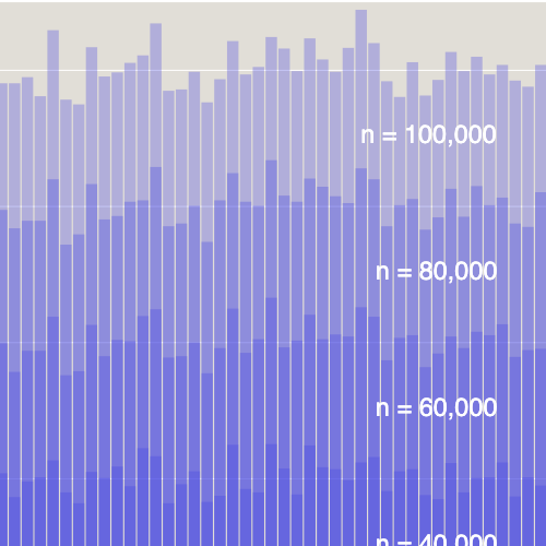
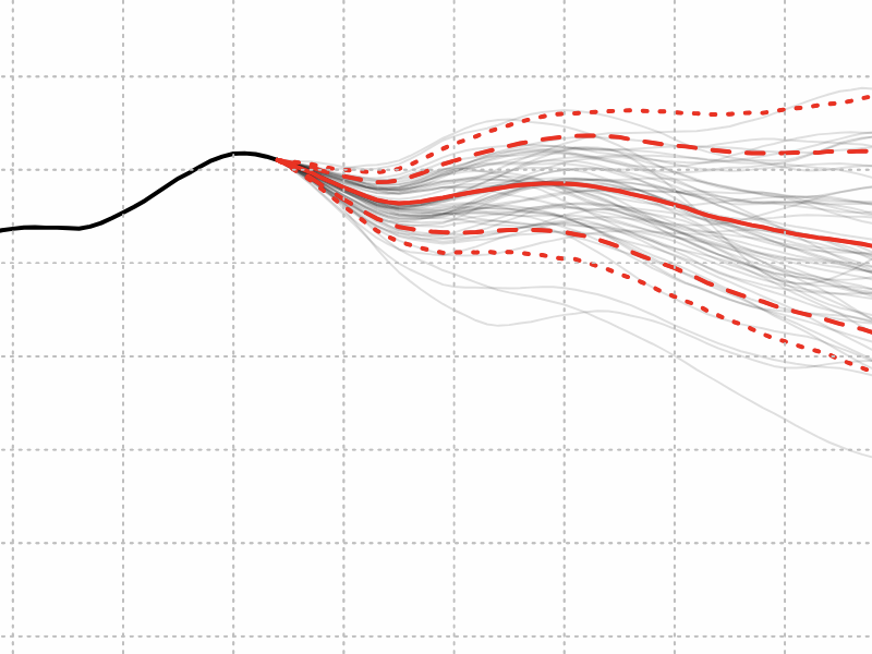
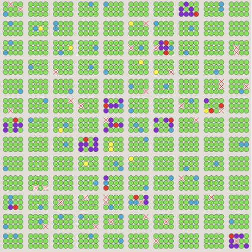
Does a greedier placement algorithm do better? If the dot positions were sampled from a left-skewed distribution, would that make it jam less?
If \(s\) is near the jamming threshold, shoving the first disk toward a corner would reduce the chance of ending the series with that disk. After the first disk, I doubt it would help. The only available spots are near the opposite corner.
At best, a nonuniform distribution could alter the efficiency of the process, not the set of feasible outcomes. Any configuration that can be reached at all will eventually by found by the random algorithm — although “eventually” might have a very large value.
Sorry to ask, but could you please write much shorter posts? The problem is that it occupies the whole space of the TCS blog aggregator your signed to, and thus disables people from seeing other blog posts. Could you please do something to fix this problem?
I am embarrassed. I’ve been behaving like the fat man in the middle seat who monopolizes both armrests. But the fact is, I had no idea I was being “aggregated.” I think there’s a technical solution, in which you aggregate only the first few sentences of the post, with a link to the rest. I’ll have to look into that.
A question: When I write a blog post like this one, with 2,000 lines of embedded JavaScript, does all that come through in the aggregated version? Do the programs run?
Yes, your post simply takes over 80% of the TCS blog aggregator http://cstheory-feed.org/
That’s an issue with your aggregator. Aggregators should work in harmony with the posts they are aggregating, not the other way around.
Brian, on the contrary please continue to write articles as long as they need to be. Do not alter your work to appease faulty aggregators. This post is great because of it’s detail.
Contrary to the previous comment I would ask you _not_ to write shorter posts. Your posts, although sadly less frequent, are always truly marvellous. I poll your site daily and when a new item appears it is like a little xmas for me. I just wanted to say thank you.
Don’t listen to the haters - I love this type of long interactive deep-dive. Thank you and keep up the good work.
2 years late but this was very interesting. Thankfully my university has the book by Shier so i can see more cool pictures :)