A Slight Discrepancy
by Brian Hayes
Published 23 June 2011

The image above shows the mesh top of a patio table, photographed after a soaking rain. Some of the openings in the mesh retain drops of water. What can we say about the distribution of those drops? Are they sprinkled randomly over the surface? The rainfall process that deposited them certainly seems random enough, but to my eye the pattern of occupied sites in the mesh looks suspiciously even and uniform.
For ease of analysis I have isolated a square piece of the tabletop image (avoiding the central umbrella hole), and extracted the coordinates of all the drops within the square. There are 394 drops, which I plot below as blue dots:

Again: Does this pattern look like the outcome of a random process?
I come to this question in the aftermath of writing an American Scientist column that explores two varieties of simulated randomness: pseudo and quasi. Pseudorandomness needs no introduction here. A pseudorandom algorithm for selecting points in a square tries to ensure that all points have the same probability of being chosen and that all the choices are independent of one another. Here’s an array of 394 pseudorandom dots constrained to lie on a skewed and rotated lattice somewhat like that of the mesh tabletop:

Quasirandomness is a less familiar concept. In selecting quasirandom points the aim is not equiprobability or independence but rather equidistribution: spraying the points as uniformly as possible across the area of the square. Just how to achieve this aim is not obvious. For the 394 quasirandom dots shown below, the x coordinates form a simple arithmetic progression, but the y coordinates are permuted by a digit-twiddling process. (The underlying algorithm was invented in the 1930s by the Dutch mathematician J. G. van der Corput, who worked with one-dimensional sequences, and extended to two dimensions in the 1950s by K. F. Roth. For more details, see my American Scientist column, page 286, or the splendid book by Jiri Matousek.)

Which of these point sets, the pseudo or the quasi, is a better match for the raindrops? Here are the three patterns in miniature, placed side-by-side as an aid to comparison:

Each of the panels has a distinctive texture. The pseudorandom pattern has both tight clusters and large voids. The quasirandom dots are more evenly spaced (though there are several close pairs of points), but they also form distinctive, small-scale repetitive motifs, most notably a hexagonal structure that repeats with not-quite-crystalline regularity. As for the raindrops, they appear to be spread over the area at almost uniform density (in this respect resembling the quasirandom pattern), but the texture shows hints of swirly rather than latticelike structures (more like the pseudorandom example).
Rather than just eyeballing the patterns, we could try a quantitative approach to describing or classifying them. There are lots of tools for this purpose—radial distribution functions, nearest-neighbor statistics, Fourier methods—but my main motive for bringing up this question in the first place is to play with a new toy that I learned about in the course of reading up on quasirandomness. It is a quantity called discrepancy, which attempts to measure how much a point set departs from a uniform spatial distribution.
There are lots of variations on the concept of discrepancy, but I’m going to discuss just one measurement scheme. The idea is to superimpose rectangles of various shapes and sizes on the pattern, allowing only rectangles with sides parallel to the x and y axes. Here are three example rectangles drawn on the raindrop pattern:

Now count the number of dots enclosed by each rectangle, and compare it with the number of dots that would be enclosed—based on the rectangle’s area—if the distribution of dots were perfectly uniform throughout the square. The absolute value of the difference is the discrepancy D(R) associated with rectangle R:
D(R) = | N · area(R) – #(P ∩ R) |,
where N is the total number of dots and #(P ∩ R) denotes the number of dots P in rectangle R. For example, the rectangle at the upper left covers 10 percent of the area of the square, so its fair share of dots would be 0.1 × 394 = 39.4 dots. The rectangle actually encloses only 37 dots, and so the discrepancy associated with the rectangle is |39.4 — 37| = 2.4. Note that the density of dots in the rectangle could be either higher or lower than the overall average; in either case the absolute-value operation would give a positive discrepancy.
For the pattern as a whole, we can define the global discrepancy D as the worst-case value of this measure, or in other words the maximum discrepancy taken over all possible rectangles drawn in the square. Van der Corput asked whether point sets could be constructed with arbitrarily low discrepancy, so that D would always remain below some fixed bound as N goes to infinity. The answer is No, at least in one and two dimensions; the minimal growth rate is O(log N). Pseudorandom patterns generally have even higher discrepancy, O(√N).
How can you find the rectangle that has maximum discrepancy for a given point set? When I first read the definition of discrepancy, I thought it would be impossible to compute exactly, because there are infinitely many rectangles to be considered. But after thinking about it a while, I realized there are only finitely many candidate rectangles that might possibly maximize the discrepancy. They are the rectangles in which each of the four sides passes through at least one dot. (Exception: Candidate rectangles can also have sides lying on the boundary of the enclosing square.)
Suppose we encounter the following rectangle:

The left, top and bottom sides each pass through a dot, but the right side lies in “empty space.” This configuration cannot be the rectangle of maximum discrepancy. We could push the right edge leftward until it just intersects a dot:

This change in shape reduces the area of the rectangle without altering the number of dots enclosed, and thus increases the density of dots. Alternatively, we could push the edge the other way:

Now we have increased the area, again without changing the count of enclosed dots, and thereby lowered the density. At least one of these actions must increase D(R), compared with the initial configuration. Thus every rectangle with all four sides touching dots or the edges of the square is a local maximum of the discrepancy function; by enumerating all rectangles in this finite set, we can find the global maximum.
There is also the irksome question of whether the rectangle is to be considered “closed” (meaning that points on the boundary are included in the area) or “open” (boundary points are excluded). I’ve sidestepped that problem by tabulating results for both open and closed boundaries. The closed form gives the highest discrepancy for densely populated rectangles, and the open form maximizes discrepancy for sparsely populated rectangles.
By considering only extrema of the discrepancy function, we make the counting problem finite—but not easy! In a square with N dots (all with distinct x and y coordinates), how many rectangles have to be considered? This turns out to be a really sweet little problem, with a simple combinatorial solution. I’m not going to reveal the answer here, but if you don’t feel like working it out for yourself, you could look it up in the OEIS or see a short paper by Benjamin, Quinn, and Wurtz. What I will say is that for N = 394, the number of rectangles is 6,055,174,225—or double that if you count open and closed rectangles separately. For each rectangle, it’s necessary to figure out how many of the 394 points are inside and how many are outside. Pretty big job.
One way to reduce the computational burden is to retreat to a simpler measure of discrepancy. Much of the literature on quasirandom patterns in two or more dimensions uses a quantity called star discrepancy, or D*. The idea is to consider only rectangles “anchored” at the lower left corner of the square (which we can conveniently identify with the origin of the xy plane). In this case the number of rectangles is just N2, or about 150,000 for N = 394.
Here is the rectangle that defines the global star discrepancy of the raindrop pattern:

The dark green rectangle at the bottom covers about 55 percent of the square and ought to encompass 216.9 dots, if the distribution were truly uniform. The actual number of dots included (assuming a “closed” rectangle) is 238, for a discrepancy of 21.1. No other rectangle anchored to the corner (0,0) has a greater discrepancy. (Note: Because of limited graphic resolution, the D* rectangle appears to extend horizontally all the way across the unit square; in fact the right edge lies at x = 0.999395.)
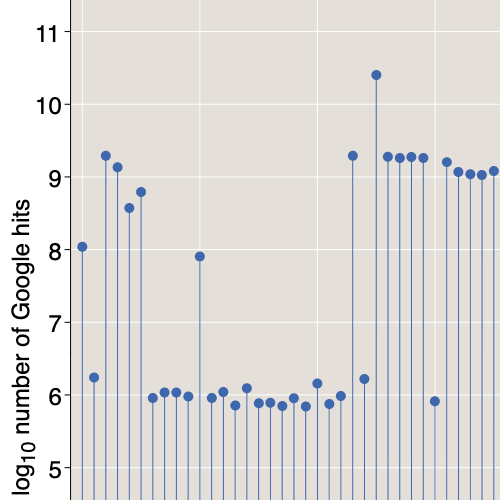
What does this result tell us about the nature of the raindrop pattern? Well, for starters, the discrepancy is fairly close to √N (which is 19.8 for N = 394) and not particularly close to log N (which is 6.0 for natural logs). Thus we get no support for the idea that the raindrop pattern might be more quasirandom than pseudorandom. The D* values for the other patterns shown above are in the ranges expected: 25.9 for the pseudorandom and 4.4 for the quasirandom. Contrary to the visual impression, the raindrop distribution seems to have more in common with a pseudorandom point set than a quasirandom one—at least by the D* criterion.
What about calculating the unrestricted discrepancy D—that is, looking at all rectangles rather than just the anchored rectangles of D*? A moment’s thought shows that this exhaustive enumeration of rectangles can’t change the basic conclusion in this case; D can never be less than D*, and so we can’t hope to move from √N toward log N. But I was curious about the computation anyway. Among those six billion rectangles, which one has the greatest discrepancy? Is it possible to answer this question without heroic efforts?
The obvious, straightforward algorithm for D generates all candidate rectangles in turn, measures their area, counts the dots inside, and keeps track of the extreme discrepancies seen along the way. I found that a program implementing this algorithm could determine the exact discrepancy of 100 pseudorandom or quasirandom dots in a few minutes. This outcome might seem to offer some encouragement for pushing on to higher N; however, the running time almost doubles every time N increases by 10, which suggests the computation would take a couple of centuries at N = 394.
I’ve invested a few days’ work in efforts to speed up this calculation. Most of the running time is spent in the routine that counts the dots in each rectangle. Deciding whether a given dot is inside, outside or on the boundary takes eight arithmetic comparisons; thus, at N = 394, there are more than 3,000 comparisons for each of the six billion rectangles. The most effective time-saving device I’ve discovered is to precompute all the comparisons. For each point that can become the lower left corner of a rectangle, I precompute a list of all the pattern dots above and to the right. For each potential upper right corner of a rectangle, I compile a similar list of dots below and to the left. These lists are stored in a hash table indexed by the corner coordinates. Given a rectangle, I can then count the number of interior dots just by taking the set intersection of the two lists.
With this trick, the estimated running time for N = 394 came down from two centuries to about two weeks. A big improvement—just enough encouragement to induce me to spend yet another day on further refinements. Replacing the hash table with an N × N array helped a little. And then I figured out a way to ignore all the smallest rectangles, those that cannot possibly be the max-D rectangle because they either contain too few dots or have too small an area. This improvement finally brought the running time down to the overnight range. The illustration below, which shows the rectangle of maximum discrepancy D for the raindrop pattern, took six hours to compute.

The max-D rectangle is clearly a slight refinement of the D* rectangle for the same point set. The D rectangle “should” contain 204.3 dots but actually has 229, for a discrepancy of D = 24.7. Of course knowing that the exact discrepancy is 24.7 rather than 21.1 tells us nothing more about the nature of the raindrop pattern. As a matter of fact, I feel I know less and less about it as I compute more and more.
When I started this project, I had a pet theory about what might be happening in the tabletop to smooth out the distribution of drops and thereby make the pattern look more quasi- than pseudorandom. To begin with, think of droplets lying on a smooth pane of glass rather than a metal mesh. If two small droplets come close enough to touch, they merge into one larger drop, because that configuration has lower energy associated with surface tension. Perhaps something similar could happen in the mesh. If two adjacent cells of the mesh are both filled with water, and if the metal channel between them is wet, then water could flow freely from one drop to the other. The larger drop will almost surely grow at the expense of the smaller one, and the latter will eventually be annihilated. Thus we would expect a deficit of drops in adjacent cells, compared with a purely random distribution.
This idea still sounds pretty good to me. The only trouble is: It explains a phenomenon that may not exist. I don’t know whether my discrepancy measurements actually reveal anything important about the three patterns, but at the very least the measurements fail to provide evidence that the raindrop distribution is different from the pseudorandom distribution. True, the patterns look different, but how much should we trust our perceptual apparatus in a case like this? If you ask people to draw dots at random, most do a bad job of it, typically making the distribution too smooth and even. Maybe the brain is equally challenged when trying to recognize randomness.
Nevertheless, I suspect there is some mathematical property that will more effectively distinguish between these patterns. If anyone else would like to sink some time into the search, the xy coordinates for the three point sets are in a text file here.
Update 2011-06-24: This is just a brief note to suggest that if you’ve read this far, please go on and read the comments, too. There’s much of value there. I want to thank all those who took the trouble to propose alternative explanations or algorithms, and to point out weaknesses in my analysis. Special thanks to themathsgeek, who within 40 minutes after I first posted the item had come up with a far superior program for computing discrepancies. Also Iain, who pursued my offhand remarks about the perception of random patterns with actual experiments.
Responses from readers:
Please note: The bit-player website is no longer equipped to accept and publish comments from readers, but the author is still eager to hear from you. Send comments, criticism, compliments, or corrections to brian@bit-player.org.
Publication history
First publication: 23 June 2011
Converted to Eleventy framework: 22 April 2025
Instead of pre-computing all the comparisons to speed up the calculation, would it not make sense to sort all the points into two arrays. I one array they would be sorted by increasing x-coordinate, in the other by increasing y-coordinate. In this way you would immediately know how many points are inside the rectangle without actually counting them.
Some thoughts on this problem:
1. What if the distribution grid that is important does not have the same cell size as the wire mesh?
2. I wonder if the distribution is partly determined by the strike energy of the raindrops? That is, a raindrop striking the grid has a certain chance of dislodging raindrops in the adjacent cells. This would suggest that it leans towards quasi-randomness. Let’s call the distance, in cells, where this has a 50% chance LD50
3. It would be interesting to compare the actual distribution to a grid of cell size LD50, where points are jiggled around the center of the cell by the poisson distribution.
OK. I’ve had a go at writing a code to find the maximum discrepancy of any point set. For the 394 points from the example it takes about 4.4 seconds on my computer to get D=24.7349. The code can be found here http://bit.ly/jynMsw
@Not a math geek: As to your point 2. I think it is more to do when the raindrops fall from the table after the rain has stopped. The drop that is dripping off the table will probably suck up some of the water around it in order to gain enough weight by capillary forces. This might create the empty holes.
@themathsgeek:
Bravo!
But I’m not quite sure I understand what you’re doing. Your data structure tells you how many points are above or below a line, or how many are to the left and the right, but to count the points inside a rectangle you need the intersection of four such values, no? I don’t see where in the code that’s happening. Perhaps I misunderstand what you were suggesting in your first comment.
In any case, you got the right answer (within the expected precision), so you must be doing something right!
By the way, what are the coordinates of the max-D rectangle?
So you give your answer right in your third last paragraph. You have a model: cells near filled cells will be full with less probability then randomly picked cells. You don’t need discrepancy to calculate this. You can just check it. Then check it vs some given pseudorandom distribution. You can probably analytically calculate what the difference would be for pseudorandom distributions.
This problem is very similar to what is done to check PNRG’s. There you look at more than just 2-d, I used to check up to 7 or 8 dimensions to see if there were any patterns (stripes).
@brian:
In the outer loop I iterate through all the points in the array where the points are sorted in the x-direction. I always know exactly which points are in my x-interval and I have marked them (setting marked=true).
Before I call the inner loop, I copy all the marked points to subSetY, but I copy them from the sortY array. This has the effect that subSetY contains all the points in the x-interval but sorted in the y-direction.
In the inner loop, I can repeat the same procedure as in the outer loop, but only on the subSetY array. The inner loop successively tests all available y-intervals on this sub-set of points. All the points selected in this way have to lie inside the rectangle.
The coordinates of the max-D rectangle are (0.02421,0.01937) -(0.99949, 0.55095)
Updated code (use this link for the most current revision) http://bit.ly/miambN
You can’t compare root(N) or log(N) to your D/D* because you don’t know what the constants are!
For algorithms for computing discrepancy of point sets efficiently using geometric data structures, see Computing the discrepancy with applications to supersampling patterns. D. P. Dobkin, D. Eppstein, and D. P. Mitchell. ACM Trans. on Graphics 15(4):354-376, 1996. http://doi.acm.org/10.1145/234535.234536
The rectangle discrepancy described in section 3 of that paper is only for rectangles having one corner at the origin but likely the same techniques can be used to speed up the arbitrary-rectangle discrepancy you consider here.
Since the table mesh is closer to a hexagonal mesh than a square one, it may make sense to use either a hexagon, a triangle or parallelogram with suitable angles and side lengths in the calculation of discrepancy. In particular, the computation for a parallelogram would be the same as that for a rectangle up to a coordinate transform in the input.
The pet theory you have about the distribution sounds similar to what a cellular automaton would do. In fact, the results of running Conway’s Game of Life from a random pattern to a stable/oscillatory state give a large-scale pattern that seems to be distributed somewhat like the quasi-random pattern. Of course, the eventual distribution coming from a CA would depend on which rule is used, but it is possible that the physics behind the raindrop pattern can be modeled by a suitable CA rule. While this approach seems promising, there are clearly way too many possibilities to try them all.
I would also like to point out that if you leave the same table on its side in the rain, you will get what appears to be almost the same type of pattern. Can the effect of gravity can be detected through the kind of point-set measuring techniques described?
Perhaps you could learn something from the alpha shape filtration of the point clouds.
The eye will tend to see patterns where there are none (as in the stars), and will tend to see no patterns when there is one, specifically the pattern of “dots eat other dots near them”. I think it was in one of Stephen Jay Gould’s essays that I first read about this: a cave full of luminescent critters hanging from the ceiling, which the guide compared to the heavens, but which Gould said had far too little visible pattern to look like the actual sky. In this case, no two critters could be too close together.
The simulated pseudo pattern might need tweaking for comparison to the raindrop distbn. The raindrops are constrained to lie on a finite set of points (the holes in the grid). Your rain drop co-ordinates are presumably the centers of a filled hole in the grid? The size of the gaps between hole centers (the grid size) will induce the self-repelling/declustering effect if you’re looking at a small area of the grid even if the filled holes are uniformly distributed.
As usual, this blog is excellent.
I don’t think the issue here is “quasi” vs “pseudo”. The water droplets are random. The question is whether they are uniform at random or drawn from a process with interactions.
Regarding: “True, the patterns look different, but how much should we trust our perceptual apparatus in a case like this?”. It’s easy to construct formal statistical tests out of human judgements (Buja et al., 2009). Generate 19 simulated patterns and give them to someone along with the real pattern. Ask them to pick an “odd-one-out” — if they identify the real data, you can reject the null hypothesis that the data came from the same distribution as your model (with p=0.05 significance). If you need a test with greater power, use more subjects.
For a test to make sense with the quasi-random numbers, you’d need a randomized version of that model. However, without defining a full distribution, you don’t have a proper generative model for the data anyway.
@article{buja2009,
title={Statistical inference for exploratory data analysis and model diagnostics},
author={Andreas Buja and Dianne Cook and Heike Hofmann and Michael Lawrence and Eun-Kyung Lee},
journal={Phil. Trans. R. Soc. A},
volume={367},
pages={4361–4383},
year={2009},
url={http://rsta.royalsocietypublishing.org/content/367/1906/4361.full.pdf}
}
When I plotted 19 uniform-at-random sets of 394 points and shuffled them with the data, I could spot the real data immediately.
I then dropped points one at a time onto a 60×60 grid, removing any points in the 8-neighborhood of each new point, until I had 394 points. Again, I simulated 19 data sets and shuffled in the real one. I could eventually spot the real data, because there were no points in a perfect horizontal line. It was hard though. If I did a simulation on the same jiggled hexagonal grid as your data, I don’t think I would spot the data from the fakes.
@billb
If we’re just comparing results at a single value of N, we don’t really need to know the constants or the rates of growth.
As it happens, though, I do have some pretty strong hints about what the constants are. They appear to be of order unity. To a fair approximation, the discrepancy of N pseudorandom points in two dimensions is 1.6 * sqrt(N). For N quasirandom points the discrepancy is very close to 1.0 * log(N). These are empirically determined values.
@ D. Eppstein,
Thanks much for the reference to your ToG paper from 1996. I had not come across it in my earlier reading, which is too bad because it gives a particularly lucid account of algorithms for computing discrepancy.
I have not done a comprehensive check of bibliographies, but I get the sense that many of the mathematicians working on low-discrepancy sequences are not regular readers of Transactions on Graphics. Among the works I have ready at hand, only one cites your paper.
Some references to work on human perception of random sequences:
Randomness and Coincidences: Reconciling Intuition and Probability theory by Thomas L. Griffiths , Joshua B. Tenenbaum,
Beliefs about what types of mechanisms produce random sequences by D. S. Blinder and
Effective Generation of Subjectively Random Binary Sequences by Yasmine B. Sanderson.
I think one reason you get a larger discrepancy than for quasirandom numbers could be that the density isn’t constant, e.g. due to physical properties of the table (tilting, variation in the size of the openings, …). For example, if the density of dots systematically increases as you move down in the square, I guess that the worst rectangle would probably be a large part of the lower (or upper) half of the square (like the one you obtained), and the discrepancy would be higher than in the case of constant density with the same total number of dots.
I’m nothing on the maths, but is it possible, if they’re just being held by surface tension, that the impact of raindrops has a chance of knocking other, nearby drops already held in the mesh out, thereby having a density-limiting effect?
The discrepancy arises because you are looking at two dimensional distribution of something that is three dimensional in nature. The rain drops are formed in clouds which are three dimensional, you are taking a two dimensional sample. You wold encounter even more discrepancy if you just sample along a single line, rather than a plane.
To expand upon my earlier comment, consider a 100 cm^2 two dimensional sample of rain fall. Assuming that there is no wind, the rain fall is produced by condensation of moisture in region which has volume : 10 cm x 10 cm x h cm, Where h is the height of the cubic region. Generally since h >> 1 cm. There exist numerous factors such as temperature gradient, variation in composition which govern the amount of condensation, and thus the distribution of the rain drops. Thus an ideal random model would simulate formation of rain drops in three dimensions, and then look at the cumulative distribution in a two dimensional cross section. I think that above effects would contribute much more to distribution of rain drops than the structure of the mesh.
For anything like this you need to somehow consider the scales involved… if the pattern of raindrops is affected by some short range interaction, like water flowing from one cell to another, measuring the global discrepancy is probably not the best way to show such effects.
Hmm, you could subdivide each pattern into grids of various sized squares, and compute the average discrepancy of each set. And then plot this average discrepancy against the grid size. (Perhaps with some sort of normalization?)
I would guess that something interesting would emerge from the raindrop pattern — evidence of some physical effect associated with a particular scale. (Cell seperation?) Whereas of course the pseudo-random pattern should be insensitive to scale.
I’m here via Hacker News, and I’ll repeat a comment I made there.
At first glance, how I’d find the maximum:
1. Reorient the cells from paralellograms to squares, with integer coordinates.
2. Create lookup tables, with dots from the origin to a given (x, y).
3. Any given rectangle:
A BC Dhas a count given by the lookup tables for B and C, minus A and D.
4. Then, iterate over all the rectangles.
I guess with a set this sparse, you could numerate all the useful x and y to check, and skip step 1.My guess for the mechanism is uneven heat dissipation. The metal stores and conducts heat, and the liquid water serves as a heat sink until it reaches its heat-sink capacity and evaporates.
After the rain, as the metal table top warms by uniform radiant heating, variations in water volume will result in one cell evaporating first. At that point, the surrounding metal will heat faster, so water holes will tend to grow.
That doesn’t really explain the pattern very well, but that was the first guess that came to mind.
Akshay is right, I think.
It is *not* a correct assumption that the formation of raindrops are independent events.
If you take a column 1cm x 1cm that cuts through the cloud, there is a limited amount of moisture in that column. It cannot spawn raindrops indefinitely, which is perfectly possible in the pseudorandom generation.
If, as a quick google search indicates, raindrops are formed around seed particles in the air (dust, smoke, etc) then their formation may well be dictated by the diffusion of such particles, which would suggest an even distribution rather than a random one.
This is no more of a guess than any of the questions around, “What happens when raindrops hit the table (do they splatter?) ” but in general I think the physical constraints around raindrop formation mean that it’s not really random, after all.
I don’t think that matters too much, Scott, because the clouds where the rain forms are typically not stationary.
There are any number of plausible sounding stories for how these things are generated, but without feedback from data, chances are they’re all wrong! :)
I took your datasets and tried plotting them in many different ways (using IPython/PyLab), after some false starts (as well as recreating your discrepancy measurements) I came up with a very simple visualisation that (IMO) beautifully shows the differences in distributions between the pseudo-random (restricted to grid), quasi-random, raindrop measurements and pseudo-random (uniform) datasets.
The plot and my explanation of it is a bit long for this blog-comment so I did a little write-up here: http://devio.us/~tripzilch/raindrops/
Hope you like it :-)
Readers of this fun posting may further enjoy Bernard Chazelle’s The Discrepancy Method: Randomness and Complexity, available in PDF from his website: http://www.cs.princeton.edu/~chazelle/
From the preface:
Interestingly, the final sentence in the above quote is contrary to the linked American Scientist column from this posting, where Brian writes in the next to last paragraph, “An open question is whether every algorithm can be derandomized. Deep thinkers believe the answer will turn out to be yes.” I have taken both quotes out of their contexts though. Further reading reveals that discrepancy has interesting things to say about this question.
Ah, now that I am about to post this I see that Chazelle’s book is already mentioned in the column’s bibliography. Consider this comment then as an endorsement to hoard free textbooks whenever possible.
But how best could you simulate the real raindrops? Clearly neither the pseudo nor quasi-random simulations quite approach the real data. What if you were to use a hybrid? I.E. Run two separate simulations, find the closest set of pairs between the two, then average the two. Well, I suppose you could create a whole new randomization algorithm for points in n dimensions weighted to a particular input discrepancy, theoretically, at any rate.
When you say that your discrepancy is close to sqrt(N), that is not itself a relevant statement. What is important is the change in discrepancy with increasing N. In other words, as N increases toward infinity, how does D change? If it changes logarithmically, that would be good evidence that the distribution is quasirandom. You state that 24 isn’t particularly close to log(N) for natural log, but what makes natural log special? For example, if you used log base ~1.27, then D is approximately equal to log(N).
Ahh I hadn’t seen your response to brian above. In that case, I’m out of ideas
I think the discussion about the randomness of raindrops’ creation is not really relevant. Even if there exists a valid theory that gives a correct result, it is not at all clear how this can in turn say something about the distribution of the droplets. One easy experiment that can be done to see if the raindrops have any effect is to pour smoothly water on the grid, let it drain and check the distribution. I believe that the air blowing through the holes has a much greater effect.
So I think that it only makes sense to see this system as a cellular automaton and try to figure out its rule. This means of course that everything should be done on a hexagonal grid.
tripzilch’s analysis hints that. We see that a droplet rarely has a close neighbor. Maybe one should try to create a uniform random distribution of points but with the rule that a point cannot be placed too close (whatever this may mean) to any other and check the result against the data.
Is it then safe to say that what the eye perciefs random as orderly which would mean that orderly is realy random?
gr Gouwerijn
I am, by no means a mathimitician or dabbler in said science, but I have to ask this. Does your equation take into account outside wind variables or the splash effect of the droplets? I find this all fascinating and thank you for the article.