Questions About Trees
by Brian Hayes
Published 4 September 2020
 “The woods are lovely, dark and deep,” wrote Robert Frost. Those iambs come to me unbidden every time I set off down a nearby woodland trail. The trail is named for Frost, who spent several years in this part of Massachusetts, teaching boys in brass-buttoned blazers at Amherst College. Did the poet ever stroll among these particular trees? It’s possible, though they would have been saplings then, a century ago. In any case, if he stopped by these woods, he didn’t stay. He had promises to keep, and miles to go before he would sleep.
When I follow Frost’s trail, it leads me into an unremarkable patch of Northeastern woodland, wedged between highways and houses and the town dump. It’s nowhere dark and deep enough to escape the sense of human proximity. This is not the forest primeval. Still, it is woodsy enough to bring to mind not only the rhymes of overpopular poets but also some tricky questions about trees and forests—questions I’ve been poking at for years, and that keep poking back. Why are trees so tall? Why aren’t they taller? Why do their leaves come in so many different shapes and sizes? Why are the trees trees (in the graph theoretical sense of that word) rather than some other kind of structure? And then there’s the question I want to discuss today:
Taking a quick census along the Frost trail, I catalog hemlock, sugar maple, at least three kinds of oak (red, white, and pin), beech and birch, shagbark hickory, white pine, and two other trees I can’t identify with certainty, even with the help of a Peterson guidebook and iNaturalist. The stand of woods closest to my home is dominated by hemlock, but on hillsides a few miles down the trail, broadleaf species are more common. The photograph below shows a saddle point (known locally as the Notch) between two peaks of the Holyoke Range, south of Amherst. I took the picture on October 15 last year—in a season when fall colors make it easier to detect the species diversity.

Forests like this one cover much of the eastern half of the United States. The assortment of trees varies with latitude and altitude, but at any one place the forest canopy is likely to include eight or ten species. A few isolated sites are even richer; certain valleys in the southern Appalachians, known as cove forests, have as many as 25 canopy species. And tropical rain forests are populated by 100 or even 200 tall tree species.
From the standpoint of ecological theory, all this diversity is puzzling. You’d think that in any given environment, one species would be slightly better adapted and would therefore outcompete all the others, coming to dominate the landscape. Garrett Hardin has written on the provenance of the principle. The mathematical formulation should probably be attributed to Vito Volterra.Ecologists call this idea the principle of competitive exclusion. It states that two or more species competing for the same resources cannot coexist permanently in the same habitat. Eventually, all but one of the competitors will be driven to local extinction. Trees of the forest canopy do seem to compete for the same resources—sunlight, CO2, water, various mineral nutrients—so the persistence of mixed-species woodlands begs for explanation.
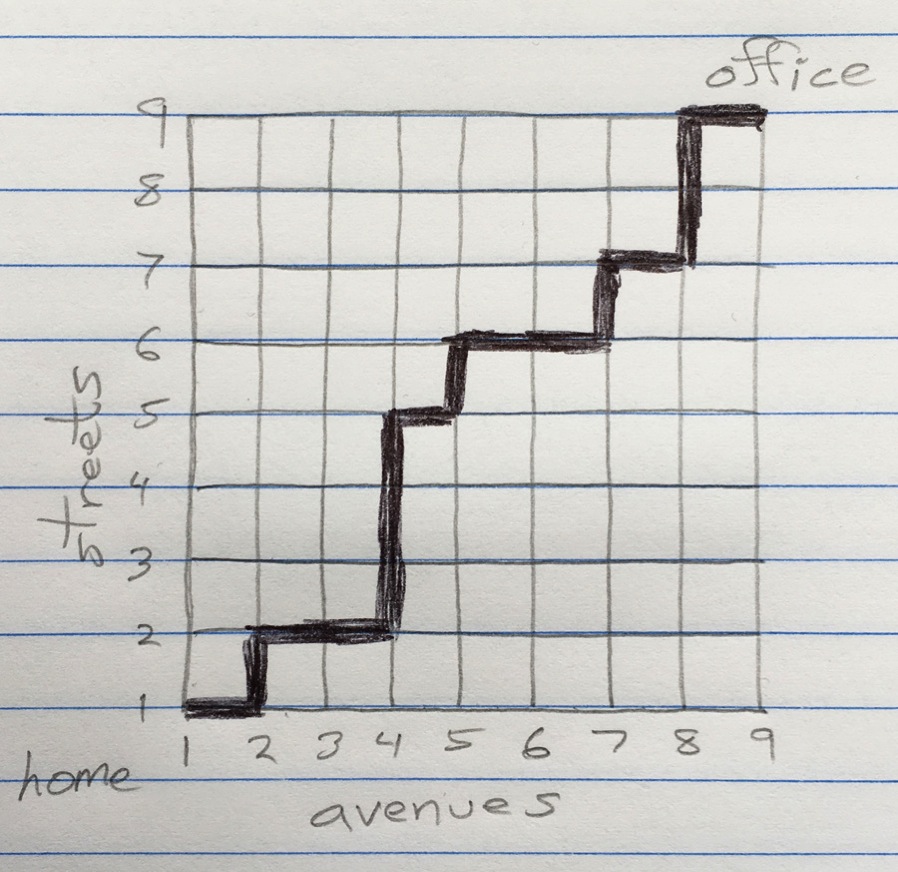
Here’s a little demo of competitive exclusion. Two tree species—let’s call them olive and orange—share the same patch of forest, a square plot that holds 625 trees.
Source code for the six computer simulations in this article is available on GitHub.
Initially, each site is randomly assigned a tree of one species or the other. When you click the Start button (or just tap on the array of trees), you launch a cycle of death and renewal. At each time step, one tree is chosen—entirely at random and without regard to species—to get the axe. Then another tree is chosen as the parent of the replacement, thereby determining its species. This latter choice is not purely random, however; there’s a bias. One of the species is better adapted to its environment, exploiting the available resources more efficiently, and so it has an elevated chance of reproducing and putting its offspring into the vacant site. In the control panel below the array of trees is a slider labeled “fitness bias”; nudging it left favors the orange species, right the olives.
The outcome of this experiment should not come as a surprise. The two species are playing a zero-sum game: Whatever territory olive wins, orange must lose, and vice versa. One site at a time, the fitter species conquers all. If the advantage is very slight, the process may take a while, but in the end the less-efficient organism is always banished. (What if the two species are exactly equal? I’ll return to that question in a moment, but for now let’s just pretend it never happens. And I have deviously jiggered the simulation so that you can’t set the bias to zero.)
Competitive exclusion does not forbid all cohabitation. Suppose olive and orange rely on two mineral nutrients in the soil—say, iron and calcium. Assume both of these elements are in short supply, and their availability is what limits growth in the populations of the trees. If olive trees are better at taking up iron and oranges assimilate calcium more effectively, then the two species may be able to reach an accommodation where both survive.
In this model, neither species is driven to extinction. At the default setting of the slider control, where iron and calcium are equally abundant in the environment, olive and orange trees also maintain roughly equal numbers on average. Random fluctuations carry them away from this balance point, but not very far or for very long. The populations are stabilized by a negative feedback loop. If a random perturbation increases the proportion of olive trees, each one of those trees gets a smaller share of the available iron, thereby reducing the species’ potential for further population growth. The orange trees are less affected by an iron deficiency, and so their population rebounds. But if the oranges then overshoot, they will be restrained by overuse of the limited calcium supply.
Moving the slider to the left or right alters the balance of iron and calcium in the environment. A 60:40 proportion favoring iron will shift the equilibrium between the two tree species, allowing the olives to occupy more of the territory. But, as long as the resource ratio is not too extreme, the minority species is in no danger of extinction. The two kinds of trees have a live-and-let-live arrangement.
In the idiom of ecology, the olive and orange species escape the rule of competitive exclusion because they occupy distinct niches, or roles in the ecosystem. They are specialists, preferentially exploiting different resources. The niches do not have to be completely disjoint. In the simulation above they overlap somewhat: The olives need calcium as well as iron, but only 25 percent as much; the oranges have mirror-image requirements.
Will this loophole in the law of competitive exclusion admit more than two species? Yes: N competing species can coexist if there are at least N independent resources or environmental strictures limiting their growth, and if each species has a different limiting factor. Everybody must have a specialty. It’s like a youth soccer league where every player gets a trophy for some unique, distinguishing talent.
This notion of slicing and dicing an ecosystem into multiple niches is a well-established practice among biologists. It’s how Darwin explained the diversity of finches on the Galapagos islands, where a dozen species distinguish themselves by habitat (ground, shrubs, trees) or diet (insects, seeds and nuts of various sizes). Forest trees might be organized in a similar way, with a number of microenvironments that suit different species. The process of creating such a diverse community is known as niche assembly.
Some niche differentiation is clearly present among forest trees. For example, gums and willows prefer wetter soil. In my local woods, however, I can’t detect any systematic differences in the sites colonized by maples, oaks, hickories and other trees. They are often next-door neighbors, on plots of land with the same slope and elevation, and growing in soil that looks the same to me. Maybe I’m just not attuned to what tickles a tree’s fancy.
Niche assembly is particularly daunting in the tropics, where it requires a hundred or more distinct limiting resources. Each tree species presides over its own little monopoly, claiming first dibs on some environmental factor no one else really cares about. Meanwhile, all the trees are fiercely competing for the most important resources, namely sunlight and water. Every tree is striving to reach an opening in the canopy with a clear view of the sky, where it can spread its leaves and soak up photons all day long. Given the existential importance of winning this contest for light, it seems odd to attribute the distinctive diversity of forest communities to squabbling over other, lesser resources.
Where niche assembly makes every species the winner of its own little race, another theory dispenses with all competition, suggesting the trees are not even trying to outrun their peers. They are just milling about at random. According to this concept, called neutral ecological drift, all the trees are equally well adapted to their environment, and the set of species appearing at any particular place and time is a matter of chance. A site might currently be occupied by an oak, but a maple or a birch would thrive there just as well. Natural selection has nothing to select. When a tree dies and another grows in its place, nature is indifferent to the species of the replacement.
This idea brings us back to a question I sidestepped above: What happens when two competing species are exactly equal in fitness? The answer is the same whether there are two species or ten, so for the sake of visual variety let’s look at a larger community.
If you have run the simulation—and if you’ve been patient enough to wait for it to finish—you are now looking at a monochromatic array of trees. I can’t know what the single color on your screen might be—or in other words which species has taken over the entire forest patch—but I know there’s just one species left. The other nine are extinct. In this case the outcome might be considered at least a little surprising. Earlier we learned that if a species has even a slight advantage over its neighbors, it will take over the entire system. Now we see that no advantage is needed. Even when all the players are exactly equal, one of them will emerge as king of the mountain, and everyone else will be exterminated. Harsh, no?
Here’s a record of one run of the program, showing the abundance of each species as a function of time:

At the outset, all 10 species are present in roughly equal numbers, clustered close to the average abundance of \(625/10\). As the program starts up, the grid seethes with activity as the sites change color rapidly and repeatedly. Within the first 70,000 times steps, however, all but three species have disappeared. The three survivors trade the lead several times, as waves of contrasting colors wash over the array. Then, after about 250,000 steps, the species represented by the bright green line drops to zero population—extinction. The final one-on-one stage of the contest is highly uneven—the orange species is close to total dominance and the crimson one is bumping along near extinction—but nonetheless the tug of war lasts another 100,000 steps. (Once the system reaches a monospecies state, nothing more can ever change, and so the program halts.)
This lopsided result is not to be explained by any sneaky bias hidden in the algorithm. At all times and for all species, the probability of gaining a member is exactly equal to the probability of losing a member. It’s worth pausing to verify this fact. Suppose species \(X\) has population \(x\), which must lie in the range \(0 \le x \le 625\). A tree chosen at random will be of species \(X\) with probability \(x/625\); therefore the probability that the tree comes from some other species must be \((625 - x)/625\). \(X\) gains one member if it is the replacement species but not the victim species, an event with a combined probability of \(x(625 - x)/625\). \(X\) loses one member if it is the victim but not the replacement, which has the same probability.
It’s a fair game. No loaded dice. Nevertheless, somebody wins the jackpot, and the rest of the players lose everything, every time.
The spontaneous decay of species diversity in this simulated patch of forest is caused entirely by random fluctuations. Think of the population \(x\) as a random walker wandering along a line segment with \(0\) at one end and \(625\) at the other. At each time step the walker moves one unit right \((+1)\) or left \((-1)\) with equal probability; on reaching either end of the segment, the game ends. The most fundamental fact about such a walk is that it does always end. A walk that meanders forever between the two boundaries is not impossible, but it has probability \(0\); hitting one wall or the other has probability \(1\).
How long should you expect such a random walk to last? In the simplest case, with a single walker, the expected number of steps starting at position \(x\) is \(x(625 - x)\). This expression has a maximum when the walk starts in the middle of the line segment; the maximum length is just under \(100{,}000\) steps. In the forest simulation with ten species the situation is more complicated because the multiple walks are correlated, or rather anti-correlated: When one walker steps to the right, another must go left. Computational experiments suggest that the median time needed for ten species to be whittled down to one is in the neighborhood of \(320{,}000\) steps.
From these computational models it’s hard to see how neutral ecological drift could be the savior of forest diversity. On the contrary, it seems to guarantee that we’ll wind up with a monoculture, where one species has wiped out all others. But this is not the end of the story.
One issue to keep in mind is the timescale of the process. In the simulation, time is measured by counting cycles of death and replacement among forest trees. I’m not sure how to convert that into calendar years, but I’d guess that 320,000 death-and-replacement events in a tract of 625 trees might take 50,000 years or more. Here in New England, that’s a very long time in the life of a forest. This entire landscape was scraped clean by the Laurentide ice sheet just 20,000 years ago. If the local woodlands are losing species to random drift, they would not yet have had time to reach the end game.
The trouble is, this thesis implies that forests start out diverse and evolve toward a monoculture, which is not supported by observation. If anything, diversity seems to increase with time. The cove forests of Tennessee, which are much older than the New England woods, have more species, not fewer. And the hyperdiverse ecosystem of the tropical rain forests is thought to be millions of years old.
Despite these conceptual impediments, a number of ecologists have argued strenuously for neutral ecological drift, most notably Stephen P. Hubbell in a 2001 book, The Unified Neutral Theory of Biodiversity and Biogeography. The key to Hubbell’s defense of the idea (as I understand it) is that 625 trees do not make a forest, and certainly not a planet-girdling ecosystem.
Hubbell’s theory of neutral drift was inspired by earlier studies of the biogeography of islands, in particular the collaborative work of Robert H. MacArthur and Edward O. Wilson in the 1960s. Suppose our little plot of \(625\) trees is growing on an island at some distance from a continent. For the most part, the island evolves in isolation, but every now and then a bird carries a seed from the much larger forest on the mainland. We can simulate these rare events by adding a facility for immigration to the neutral-drift model. In the panel below, the slider controls the immigration rate. At the default setting of \(1/100\), every \(100\)th replacement tree comes not from the local forest but from a stable reserve where all \(10\) species have an equal probability of being selected.
For the first few thousand cycles, the evolution of the forest looks much like it does in the pure-drift model. There’s a brief period of complete tutti-frutti chaos, then waves of color erupt over the forest as it blushes pink, then deepens to crimson, or fades to a sickly green. What’s different is that none of those expanding species ever succeeds in conquering the entire array. As shown in the timeline graph below, they never grow much beyond 50 percent of the total population before they retreat into the scrum of other species. Later, another tree color makes a bid for empire but meets the same fate. (Because there is no clear endpoint to this process, the simulation is designed to halt after 500,000 cycles. If you haven’t seen enough by then, click Resume.)

Immigration, even at a low level, brings a qualitative change to the behavior of the model and the fate of the forest. The big difference is that we can no longer say extinction is forever. A species may well disappear from the 625-tree plot, but eventually it will be reimported from the permanent reserve. Thus the question is not whether a species is living or extinct but whether it is present or absent at a given moment. At an immigration rate of \(1/100\), the average number of species present is about \(9.6\), so none of them disappear for long.
With a higher level of immigration, the 10 species remain thoroughly mixed, and none of them can ever make any progress toward world domination. On the other hand, they have little risk of disappearing, even temporarily. Push the slider control all the way to the left, setting the immigration rate at \(1/10\), and the forest display becomes an array of randomly blinking lights. In the timeline graph below, there’s not a single extinction.

Pushing the slider in the other direction, rarer immigration events allow the species distribution to stray much further from equal abundance. In the trace below, with an immigrant arriving every \(1{,}000\)th cycle, the population is dominated by one or two species for most of the time; other species are often on the brink of extinction—or over the brink—but they come back eventually. The average number of living species is about 4.3, and there are moments when only two are present.

Finally, with a rate of \(1/10{,}000\), the effect of immigration is barely noticeable. As in the model without immigration, one species invades all the terrain; in the example recorded below, this takes about \(400{,}000\) steps. After that, occasional immigration events cause a small blip in the curve, but it will be a very long time before another species is able to displace the incumbent.

The island setting of this model makes it easy to appreciate how sporadic, weak connections between communities can have an outsize influence on their development. But islands are not essential to the argument. Trees, being famously immobile, have only occasional long-distance communication, even when there’s no body of water to separate them. (It’s a rare event when Birnam Wood marches off to Dunsinane.) Hubbell formulates a model of ecological drift in which many small patches of forest are organized into a hierarchical metacommunity. Each patch is both an island and part of the larger reservoir of species diversity. If you choose the right patch sizes and the right rates of migration between them, you can maintain multiple species at equilibrium. Hubbell also allows for the emergence of entirely new species, which is also taken to be a random or selection-neutral process.
Niche assembly and neutral ecological drift are theories that elicit mirror-image questions from skeptics. With niche assembly we look at dozens or hundreds of coexisting tree species and ask, “Can every one of them have a unique limiting resource?” With neutral drift we ask, “Can all of those species be exactly equal in fitness?”
Hubbell responds to the latter question by turning it upside down. The very fact that we observe coexistence implies equality:
All species that manage to persist in a community for long periods with other species must exhibit net long-term population growth rates of nearly zero…. If this were not the case, i.e., if some species should manage to achieve a positive growth rate for a considerable length of time, then from our first principle of the biotic saturation of landscapes, it must eventually drive other species from the community. But if all species have the same net population growth rate of zero on local to regional scales, then ipso facto they must have identical or nearly identical per capita relative fitnesses.
Herbert Spencer proclaimed: Survival of the fittest. Here we have a corollary: If they’re all survivors, they must all be equally fit.
Now for something completely different.
Another theory of forest diversity was devised specifically to address the most challenging case—the extravagant variety of trees in tropical ecosystems. In the early 1970s J. H. Connell and Daniel H. Janzen, field biologists working independently in distant parts of the world, almost simultaneously came up with the same idea. The phrase “social distancing” does not appear in the work of Connell and Janzen from 50 years ago, but today it’s irresistable as a description of their theory.In tropical forests, they suggested, trees practice social distancing as a defense against contagion, and this promotes diversity.
A tropical rain forest is a tough neighborhood. Trees are under frequent attack by marauding gangs of predators, parasites, and pathogens. (Connell lumped these bad guys together under the label “enemies.”) Many of the enemies are specialists, targeting only trees of a single species. The specialization can be explained by competitive exclusion: Each tree species becomes a unique resource supporting one type of enemy.
Suppose a tree is beset by a dense population of host-specific enemies. The swarm of meanies attacks not only the adult tree but also any offspring of the host that have taken root near their parent. Since young trees are more vulnerable than adults, the entire cohort could be wiped out.  Seedlings at a greater distance from the parent should have a better chance of remaining undiscovered until they have grown large and robust enough to resist attack. In other words, evolution might favor the rare apple that falls far from the tree. Janzen illustrated this idea with a graphical model something like the one at right. As distance from the parent increases, the probability that a seed will arrive and take root grows smaller (red curve), but the probability that any such seedling will survive to maturity goes up (blue curve). The overall probability of successful reproduction is the product of these two factors (purple curve); it has a peak where the red and blue curves cross.
The Connell-Janzen theory predicts that trees of the same species will be widely dispersed in the forest, leaving plenty of room in between for trees of other species, which will have a similarly scattered distribution. The process leads to anti-clustering: conspecific trees are farther apart on average than they would be in a completely random arrangement. This pattern was noted by Alfred Russel Wallace in 1878, based on his own long experience in the tropics:
If the traveller notices a particular species and wishes to find more like it, he may often turn his eyes in vain in every direction. Trees of varied forms, dimensions, and colours are around him, but he rarely sees any one of them repeated. Time after time he goes towards a tree which looks like the one he seeks, but a closer examination proves it to be distinct. He may at length, perhaps, meet with a second specimen half a mile off, or may fail altogether, till on another occasion he stumbles on one by accident.
My toy model of the social-distancing process implements a simple rule. When a tree dies, it cannot be replaced by another tree of the same species, nor may the replacement match the species of any of the eight nearest neighbors surrounding the vacant site. Thus trees of the same species must have at least one other tree between them. To say the same thing in another way, each tree has an exclusion zone around it, where other trees of the same species cannot grow.
It turns out that social distancing is a remarkably effective way of preserving diversity. When you click Start, the model comes to life with frenetic activity, blinking away like the front panel of a 1950s Hollywood computer. Then it just keeps blinking; nothing else ever really happens. There are no spreading tides of color as a successful species gains ground, and there are no extinctions. The variance in population size is even lower than it would be with a completely random and uniform assignment of species to sites. This stability is apparent in the timeline graph below, where the 10 species tightly hug the mean abundance of 62.5:

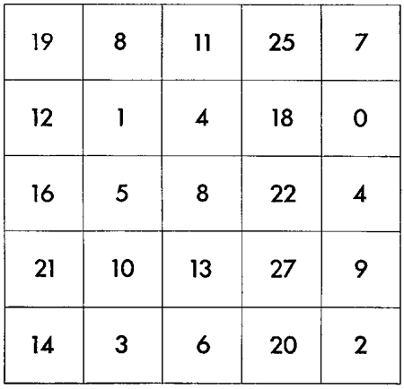
When I finished writing this program and pressed the button for the first time, long-term survival of all ten species was not what I expected to see. My thoughts were influenced by some pencil-and-paper doodling. I had confirmed that only four colors are needed to create a pattern where no two trees of the same color are adjacent horizontally, vertically, or on either of the diagonals. One such pattern is shown at right. I suspected that the social-distancing protocol might cause the model to condense into such a crystalline state, with the loss of species that don’t appear in the repeated motif. I was wrong. Although four is indeed the minimum number of colors for a socially distanced two-dimensional lattice, there is nothing in the algorithm that encourages the system to seek the minimum.
After seeing the program in action, I was able to figure out what keeps all the species alive. There’s an active feedback process that puts a premium on rarity. Suppose that oaks currently have the lowest frequency in the population at large. As a result, oaks are least likely to be present in the exclusion zone surrounding any vacancy in the forest, which means in turn they are most likely to be acceptable as a replacement. As long as the oaks remain rarer than the average, their population will tend to grow. Symmetrically, individuals of an overabundant species will have a harder time finding an open site for their offspring. All departures from the mean population level are self-correcting.
The initial configuration in this model is completely random, ignoring the restrictions on adjacent conspecifics. Typically there are about 200 violations of the exclusion zone in the starting pattern, but they are all eliminated in the first few thousand time steps. Thereafter the rules are obeyed consistently. Note that with ten species and an exclusion zone consisting of nine sites, there is always at least one species available to fill a vacancy. If you try the experiment with nine or fewer species, some vacancies must be left as gaps in the forest. I should also mention that the model uses toroidal boundary conditions: the right edge of the grid is adjacent to the left edge, and the top wraps around to the bottom. This ensures that all sites in the lattice have exactly eight neighbors.
Connell and Janzen envisioned much larger exclusion zones, and correspondingly larger rosters of species. Implementing such a model calls for a much larger computation. A recent paper by Taal Levi et al. reports on such a simulation. They find that the number of surviving species and their spatial distribution remain reasonably stable over long periods (200 billion tree replacements).
Could the Connell-Janzen mechanism also work in temperate-zone forests? As in the tropics, the trees of higher latitudes do have specialized enemies, some of them notorious—the vectors of Dutch elm disease and chestnut blight, the emerald ash borer, the gypsy moth caterpillars that defoliate oaks. The hemlocks in my neighborhood are under heavy attack by the woolly adelgid, a sap-sucking bug. Thus the forces driving diversification and anti-clustering in the Connell-Janzen model would seem to be present here. However, the observed spatial structure of the northern forests is somewhat different. Social distancing hasn’t caught on here. The distribution of trees tends to be a little clumpy, with conspecifics gathering in small groves.
Plague-driven diversification is an intriguing idea, but, like the other theories mentioned above, it has certain plausibility challenges. In the case of niche assembly, we need to find a unique limiting resource for every species. In neutral drift, we have to ensure that selection really is neutral, assigning exactly equal fitness to trees that look quite different. In the Connell-Janzen model we need a specialized pest for every species, one that’s powerful enough to suppress all nearby seedlings. Can it be true that every tree has its own deadly nemesis?
You might have to click Invade more than once, since a new arrival may die out before becoming established. Also note that I have slowed down this simulation, lest it all be over in a flash.There’s also reason to doubt the model’s robustness, its resistance to disruption. Suppose an invasive species shows up in the socially distanced tropical forest—a tree new to the continent, with no enemies anywhere nearby. What happens then? The program below offers an answer. Start it running, and then click the Invade button.
Lacking enemies, the invader can flout the social-distancing rules, occupying any forest vacancy regardless of neighborhood. Once the invader has taken over a majority of the sites, the distancing rules become less onerous, but by then it’s too late for the other species.
One further half-serious thought on the Connell-Janzen theory: In the war between trees and their enemies, humanity has clearly chosen sides. We would wipe out those insects and fungi and other tree-killing pests if we could figure out how to do so. Everyone would like to bring back the elms and the chestnuts, and save the eastern hemlocks before it’s too late. On this point I’m as sentimental as the next treehugger. But if Connell and Janzen are correct, and if their theory applies to temperate-zone forests, eliminating all the enemies would actually cause a devastating collapse of tree diversity. Without pest pressure, competitive exclusion would be unleashed, and we’d be left with one-tree forests everywhere we look.
Species diversity in the forest is now matched by theory diversity in the biology department. The three ideas I have discussed here—niche assembly, neutral drift, and social distancing—all seem to be coexisting in the minds of ecologists. And why not? Each theory is a success in the basic sense that it can overcome competitive exclusion. Each theory also makes distinctive predictions. With niche assembly, every species must have a unique limiting resource. Neutral drift generates unusual population dynamics, with species continually coming and going, although the overall number of species remains stable. Social distancing entails spatial anticlustering.
How can we choose a winner among these theories (and perhaps others)? Scientific tradition says nature should have the last word. We need to conduct some experiments, or at least go out in the field and make some systematic observations, then compare those results with the theoretical predictions.
There have been quite a few experimental tests of competitive exclusion. For example, Thomas Park and his colleagues ran a decade-long series of experiments with two closely related species of flour beetles. One species or the other always prevailed. In 1969 Francisco Ayala reported on a similar experiment with fruit flies, in which he observed coexistence under circumstances that were thought to forbid it. Controversy flared, but in the end the result was not to overturn the theory but to refine the mathematical description of where exclusion applies.
Wouldn’t it be grand to perform such experiments with trees? Unfortunately, they are not so easily grown in glass vials. And conducting multigenerational studies of organisms that live longer than we do is a tough assignment. With flour beetles, Park had time to observe more than 100 generations in a decade. With trees, the equivalent experiment might take 10,000 years. But field workers in biology are a resourceful bunch, and I’m sure they’ll find a way. In the meantime, I want to say a few more words about theoretical, mathematical, and computational approaches to the problem.
Ecology became a seriously mathematical discipline in the 1920s, with the work of Alfred J. Lotka and Vito Volterra. To explain their methods and ideas, one might begin with the familiar fact that organisms reproduce themselves, thereby causing populations to grow. Mathematized, this observation becomes the differential equation
\[\frac{d x}{d t} = \alpha x,\]
which says that the instantaneous rate of change in the population \(x\) is proportional to \(x\) itself—the more there are, the more there will be. The constant of proportionality \(\alpha\) is called the intrinsic reproduction rate; it is the rate observed when nothing constrains or interferes with population growth. The equation has a solution, giving \(x\) as a function of \(t\):
\[x(t) = x_0 e^{\alpha t},\]
where \(x_0\) is the initial population. This is a recipe for unbounded exponential growth (assuming that \(\alpha\) is positive). In a finite world such growth can’t go on forever, but that needn’t worry us here.
The original version of this essay (published on 4 September 2020) had serious errors in the description of the Lotka-Volterra equations. The problem was brought to my attention in a comment by Matt on 16 September. The corrected version here was published on 19 September.Let’s introduce a second species, \(y\), that obeys the same kind of growth law but has its own intrinsic reproductive rate \(\beta\). Now we can ask what happens if the two species interact. Lotka and Volterra (working independently) first considered the case where \(y\) preys upon \(x\). They proposed the following pair of equations, with interaction terms proportional to \(x y\):
\[\begin{align}
\frac{d x}{d t} &= \alpha x -\gamma x y\\
\frac{d y}{d t} &= -\beta y + \delta x y
\end{align}\]
The prey species \(x\) prospers when left to itself, but suffers as the product \(x y\) increases. The situation is just the opposite for the predator \(y\), which can’t get along alone (\(x\) is its only food source) and whose population swells when \(x\) and \(y\) are both abundant.
Competition is a more symmetrical relation: Either species can thrive when alone, and the interaction between them is negative for both parties.
\[\begin{align}
\frac{d x}{d t} &= \alpha x -\gamma x y\\
\frac{d y}{d t} &= \beta y - \delta x y
\end{align}\]
The Lotka-Volterra equations yield some interesting behavior. At any instant \(t\), the state of the two-species system can be represented as a point in the \(x, y\) plane, whose coordinates are the two population levels. For some combinations of the \(\alpha, \beta, \gamma, \delta\) parameters, there’s a point of stable equilibrium. Once the system has reached this point, it stays put, and it returns to the same neighborhood following any small perturbation. Other equilibria are unstable: The slightest departure from the balance point causes a major shift in population levels. And the really interesting cases have no stationary point; instead, the state of the system traces out a closed loop in the \(x, y\) plane, continually repeating a cycle of states. The cycles correspond to oscillations in the two population levels. Such oscillations have been observed in many predator-prey systems. Indeed, it was curiosity about the periodic swelling and contraction of populations in the Canadian fur trade and Adriatic fisheries that inspired Lotka and Volterra to work on the problem.
The 1960s and 70s brought more surprises. Studies of equations very similar to the Lotka-Volterra system revealed the phenomenon of “deterministic chaos,” where the point representing the state of the system follows an extremely complex trajectory, though it’s wandering are not random. There ensued a lively debate over complexity and stability in ecosystems. Is chaos to be found in natural populations? Is a community with many species and many links between them more or less stable than a simpler one?
Viewed as abstract mathematics, there’s much beauty in these equations, but it’s sometimes a stretch mapping the math back to the biology. For example, when the Lotka-Volterra equations are applied to species competing for resources, the resources appear nowhere in the model. The mathematical structure describes something more like a predator-predator interaction—two species that eat each other.
Even the organisms themselves are only a ghostly presence in these models. The differential equations are defined over the continuum of real numbers, giving us population levels or densities, but not individual plants or animals—discrete things that we can count with integers. The choice of number type is not of pressing importance as long as the populations are large, but it leads to some weirdness when a population falls to, say, 0.001—a millitree. Using finite-difference equations instead of differential equations avoids this problem, but the mathematics gets messier.
Another issue is that the equations are rigidly deterministic. Given the same inputs, you’ll always get exactly the same outputs—even in a chaotic model. Determinism rules out modeling anything like neutral ecological drift. Again, there’s a remedy: stochastic differential equations, which include a source of noise or uncertainty. With models of this kind, the answers produced are not numbers but probability distributions. You don’t learn the population of \(x\) at time \(t\); you get a probability \(P(x, t)\) in a distribution with a certain mean and variance. Another approach, called Markov Chain Monte Carlo (MCMC), uses a source of randomness to sample from such distributions. But the MCMC method moves us into the realm of computational models rather than mathematical ones.
Computational methods generally allow a direct mapping between the elements of the model and the things being modeled. You can open the lid and look inside to find the trees and the resources, the births and the deaths. These computational objects are not quite tangible, but they’re discrete, and always finite. A population is neither a number nor a probability distribution but a collection of individuals. I find models of this kind intellectually less demanding. Writing a differential equation that captures the dynamics of a biological system requires insight and intuition. Writing a program to implement a few basic events in the life of a forest—a tree dies, another takes its place—is far easier.
The six little models included in this essay serve mainly as visualizations; they expend most of their computational energy painting colored dots on the screen. But larger, more ambitious models are certainly feasible, as in the work of Taal Levi et al. mentioned above.
However, if computational models are easier to create, they can also be harder to interpret. If you run a model once and species \(X\) goes extinct, what can you conclude? Not much. On the next run \(X\) and \(Y\) might coexist. To make reliable inferences, you need to do some statistics over a large ensemble of runs—so once again the answer takes the form of a probability distribution.
The concreteness and explicitness of Monte Carlo models is generally a virtue, but it has a darker flip side. Where a differential equation model might apply to any “large” population, that vague description won’t work in a computational context. You have to name a number, even though the choice is arbitrary. The size of my forest models, 625 trees, was chosen for mere convenience. With a larger grid, say \(100 \times 100\), you’d have to wait millions of time steps to see anything interesting happen. Of course the same issue arises with experiments in the lab or in the field.
Both kinds of model are always open to a charge of oversimplifying. A model is the Marie Kondo version of nature—relentlessly decluttered and tidied up. Sometime important parts get tossed out. In the case of the forest models, it troubles me that trees have no life history. One dies, and another pops up full grown. Also missing from the models are pollination and seed dispersal, and rare events such a hurricanes and fires that can reshape entire forests. Would we learn more if all those aspects of life in the woods had a place in the equations or the algorithms? Perhaps, but where do you stop?
My introduction to models in ecology came through a book of that title by John Maynard Smith, published in 1974. I recently reread it, learning more than I did the first time through. Maynard Smith makes a distinction between simulations, useful for answering questions about specific problems or situations, and models, useful for testing theories. He offers this advice: “Whereas a good simulation should include as much detail as possible, a good model should include as little as possible.”
Further Reading
Ayala, F. J. 1969. Experimental invalidation of the principle of competitive exclusion. Nature 224:1076–1079.
Clark, James S. 2010. Individuals and the variation needed for high species diversity in forest trees. Science 327:1129–1132.
Connell, J. H. 1971. On the role of natural enemies in preventing competitive exclusion in some marine animals and in rain forest trees. In Dynamics of Populations, P. J. Den Boer and G. Gradwell, eds., Wageningen, pp. 298–312.
Gilpin, Michael E., and Keith E. Justice. 1972. Reinterpretation of the invalidation of the principle of competitive exclusion. Nature 236:273–301.
A history of the first 40 years. Someone needs to do the next 60.
Hardin, Garrett. 1960. The competitive exclusion principle. Science 131(3409): 1292–1297.
Hubbell, Stephen P. 2001. The Unified Neutral Theory of Biodiversity and Biogeography. Princeton, NJ: Princeton University Press.
Hutchinson, G. E. 1959. Homage to Santa Rosalia, or why are there so many kinds of animals? The American Naturalist 93:145–159.
Janzen, Daniel H. 1970. Herbivores and the number of tree species in tropical forests. The American Naturalist 104(940):501–528.
Kricher, John. C. 1988. A Field Guide to Eastern Forests, North America. The Peterson Field Guide Series. Illustrated by Gordon Morrison. Boston: Houghton Mifflin.
Levi, Taal, Michael Barfield, Shane Barrantes, Christopher Sullivan, Robert D. Holt, and John Terborgh. 2019. Tropical forests can maintain hyperdiversity because of enemies. Proceedings of the National Academy of Sciences of the USA 116(2):581–586.
Levin, Simon A. 1970. Community equilibria and stability, and an extension of the competitive exclusion principle. The American Naturalist, 104(939):413–423.
MacArthur, R. H., and E. O. Wilson. 1967. The Theory of Island Biogeography. Monographs in Population Biology. Princeton University Press, Princeton, NJ.
May, Robert M. 1973. Qualitative stability in model ecosystems. Ecology, 54(3):638–641.
Maynard Smith, J. 1974. Models in Ecology. Cambridge: Cambridge University Press.
Richards, Paul W. 1973. The tropical rain forest. Scientific American 229(6):58–67.
Schupp, Eugene W. 1992. The Janzen-Connell model for tropical tree diversity: population implications and the importance of spatial scale. The American Naturalist 140(3):526–530.
Strobeck, Curtis. 1973. N species competition. Ecology, 54(3):650–654.
Tilman, David. 2004. Niche tradeoffs, neutrality, and community structure: A stochastic theory of resource competition, invasion, and community assembly. Proceedings of the National Academy of Sciences of the USA 101(30):10854–10861.
Wallace, Alfred R. 1878. Tropical Nature, and Other Essays. London: Macmillan and Company.
Responses from readers:
Please note: The bit-player website is no longer equipped to accept and publish comments from readers, but the author is still eager to hear from you. Send comments, criticism, compliments, or corrections to brian@bit-player.org.
Publication history
First publication: 4 September 2020
Converted to Eleventy framework: 22 April 2025


For social distancing you don’t need each tree to have it’s own specialized disease. It would suffice to have only 2*log2(number of tree species) number of diseases.
If you had 8 trees and 6 disease then each tree could be infected by 3 diseases and each disease could infect 4 trees. Each tree would share at most 2 disease with a different species of tree.
If you try this it would be good to modify the suppression so that it is not absolute but instead perhaps each shared disease halves the chance that the sapling survives (otherwise a tree would only be able to have neighbors that it shares no diseases with)
Because each tree species would share more diseases with its own species than any other species you would still get frequency dependent fitness but you wouldn’t need as many diseases.
Brilliant! Never occurred to me. And the papers by Connell and Janzen give no hint that they were thinking along these lines either.
It would be worth modeling to see whether the “softer” rule will still preserve high diversity.
Whether the trees and their enemies think along these lines is another question, of course.
I tried it and it doesn’t work.
The reason it doesn’t work is that to maintain a diversity of N, you need each species to be have a fitness advantage over each of the other N-1, when it is missing from the community.
For this to happen each species must have a disease that isn’t present when that species isn’t present, which simplifies down to each species having it’s own unique disease.
Lovely article, thank you!
I am not sure I understand the Lotka and Volterra differential equation - I can’t see how the Predator population can ever fall in the definition above. Should beta be negative if y is the predator?
Thanks so much for pointing out this problem. I thought I had found a clever way to present the four possible interactions in a symmetric format. It was indeed symmetric and perhaps clever; unfortunately it was also quite wrong. I have amended the text above.
Something weird happened to the X-axis labels on the graph for the Connell-Janzen theory; they’re “02, 55, 07, 5, 100″ from left to right.
Well, the x axis legend does say “arbitrary units,” but I’ve got to agree those are too arbitrary for their own good.
Thanks for pointing out the problem. I’ll fix it.
Wow, I blew through a lot of this, ’cause I’m thinking; A forest is more than it’s trees, it’s also the fungi breaking down the dead stuff. They play a large unknown part in nutrient sharing in the forest. (and perhaps diversity.)