Traffic Jams in Javascript

Building bigger roads can make traffic worse. The usual explanation for this counter­intuitive and counterproductive outcome is that bigger roads attract bigger shopping malls, which in turn attract more cars. But that’s not the whole story. In the 1960s Dietrich Braess discovered a theoretical configuration of roadways where building a new connecting road can make everyone’s trip slower even when the number of vehicles is held constant. Conversely, closing a road in the Braess network can allow everyone to get home quicker. The behavior is weird enough to justify the term “Braess’s paradox.”

A few years ago Joel Cohen suggested to me that Braess’s paradox might make a good topic for my “Computing Science” column. I hesitated. There were already plenty of published discussions of the paradox, including excellent ones by Cohen himself, as well as a book by Tim Roughgarden (which I had reviewed for American Scientist). I didn’t think I had anything more to add to the conversation.

Lately, though, I began to consider the problem of visualizing Braess’s paradox—presenting it in such a way that you can watch individual cars navigating through the road network, rather than merely calculating average speeds and travel times. Having an opportunity to play with the model—fiddling with the knobs and switches, trying different routing algorithms—might lead to a clearer understanding of why well-informed and self-interested drivers would choose a route that winds up making everybody late for dinner.

I now have a working JavaScript model of something resembling Braess’s paradox, which I urge you to go take for a test drive. There’s an accompanying “Computing Science” column in the latest issue of American Scientist, available on the magazine website in HTML or PDF. If you’re interested in the source code, it’s on Github. Here I’m going to say a few words about the implementation of the model and what I’ve learned from it.

Adapting Braess’s mathematical model to a more mechanistic and visual medium was trickier than I had expected. The original formulation is quite abstract and not very physical; it’s closer to graph theory than to highway engineering. In the diagrams below the wide, blue roads labeled A and B never become congested; no matter how much traffic they carry, the transit time for these links is always one hour. The narrow red roads a and b offer a transit time of zero when they’re empty, but traffic slows as the load increases; if everyone crowds onto a single red link, the transit time is again one hour. As for the gold route X, this magical thoroughfare offers instantaneous transport for any number of vehicles.

The presence or absence of the X road is what triggers the paradox. Without the golden crosslink (left diagram), traffic splits equally between the Ab and aB routes, and all cars take 90 minutes to complete the trip. When the X link is opened (right diagram) all drivers favor route aXb, and everyone spends a full two hours on the road.

The essential supposition behind the paradox is that everyone follows a selfish routing policy, choosing whichever route offers the quickest trip, and ignoring all factors other than travel time. And, ironically, it’s the insistence that no one else may have a shorter trip that leaves all the drivers in a bumper-to-bump jam on route aXb, while AXB sits empty. Why? If any driver decided to defect to AXB, the departure would marginally lessen the load on aXb, giving the latter route a slight speed advantage. Under the selfish policy, the defecting driver would then have to return to aXb. It’s a stalemate.

Cars moving at infinite speed and roads with infinite capacity may be all right in a mathematical model, but they are troublesome in a simulation that’s supposed to look something like real highway traffic. Seeking a more realistic model, I settled on the road layout shown below, inspired by a diagram in a 1997 paper by Claude M. Pinchina (Braess Paradox: maximum penalty in a minimal critical network. Transportation Research A 31(5):379–388).

The topology is the same as that of Braess’s original network, but the geometry is different, and so is the relation between congestion and speed. The aim is still to get from start to end—or, rather, from Origin to Destination. The A and B road segments are again wide and insensitive to traffic congestion. The a and b roads are straighter and shorter but also narrower. With zero traffic, vehicle speed is the same on a and b as on A and B, but as traffic gets heavier, speed falls off. The analogue of the “golden road” is a short bridge at the center of the map, which has the same speed properties as A and B. In the initial configuration, the bridge is blocked off, but a mouseclick opens it. In the snapshot of the running model shown above, the bridge is open and carrying traffic.

Cars, represented by colored dots, enter the system at the Origin. At the moment of launching, each car chooses one of the available routes. If the bridge is closed, there are just two possibilities: Ab and aB. With the bridge open, drivers also have the option of the ab shortcut or the longer AB. The cars then advance along the selected roadways, governed by the speed restrictions on each segment, until they reach the Destination.

This scheme differs in several important ways from the original Braess formulation. Does it still exhibit the paradox? In other words, does the travel time increase when the bridge is opened, allowing traffic to flow over routes ab and AB? The answer is yes, for a wide range of parameter values, as shown in these outputs:

The tables show the number of vehicles choosing each route and the average time they spend on the road. (The times are measured in units of the quickest possible trip: taking the shortest route ab with zero traffic.) Note that opening up the bridge slowed down travel on all four routes. Even though the Ab and aB routes carried about 37 percent less traffic when the bridge was open, cars on those routes took 9 to 15 percent longer to complete their journeys. The ab and AB routes were even slower.

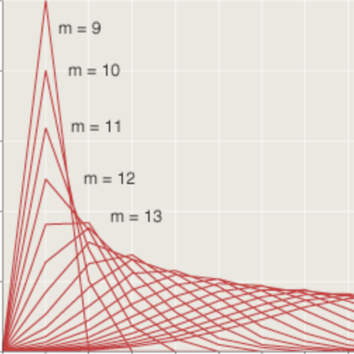
But the numbers don’t tell the whole story—that was the first thing I learned when I got the simulation running. In the bridge-closed state, where the total traffic splits into two roughly equal streams, you might imagine successive cars alternating between Ab and aB, so that the system would reach a statistical steady state with equal numbers of cars on each of the two routes at any given moment. That’s not at all what happens! The best way to see what does happen is to go run the simulation, but the graph below also gives a clue.

Instead of settling into a steady state, the system oscillates with a period of a little less than 500 times steps, which is roughly half the time it takes a typical car to make a complete trip from Origin to Destination. The two curves are almost exactly 180 degrees out of phase.

It’s not hard to understand where those oscillations come from. As each car enters the road network, it chooses the route with the shortest expected travel time, based on conditions at that moment. The main determinant of expected travel time is the number of cars occupying the a and b segments, where speed decreases as the roads get more crowded. But when cars choose the less-popular route, they also raise the occupany of that route, making it appear less favorable to the cars behind them. Furthermore, on the Ab route there is a substantial delay before the cars reach the congestion-sensitive segment. The delay and the asymmetry of the network create an instability—a feedback loop in which overshooting and overcorrection are inevitable.

When the connecting bridge is opened, the pattern is more complicated, but oscillations are still very much in evidence:

There seem to be two main alternating phases—one where Ab and ab dominate (the Christmas phase, in this color scheme), and the other where ab and AB take over (the Cub Scout phase). The period of the waves is less regular but mostly longer.

I am not the first to observe these oscillations; they are mentioned, for example, by Daniele Buscema and colleagues in a paper describing a NetLogo simulation of Braess-like road networks. Overall, though, the oscillations and instabilities seem to have gotten little attention in the literature.

The asymmetry of the layout is crucial to generating both the oscillations and the paradoxical slowdown on opening the central connecting link. You can see this for yourself by running a symmetric version of the model. It’s quite dull.

One more bug/feature of the dynamic model is worth a comment. In the original Braess network, the A and B links have unlimited capacity; in effect, the model promises that the time for traversing those roads is a constant, regardless of traffic. In a dynamic model with discrete vehicles of greater-than-zero size, that promise is hard to keep. Consider cars following the Ab route, and suppose the b segment is totally jammed. At the junction where A disgorges onto b, cars have nowhere to go, and so they spill back onto the A segment, which can therefore no longer guarantee constant speed.

In implementing the dynamic model, I discovered there were a lot of choices to be made where I could find little guidance in the mathematical formulation of the original Braess system. The “queue spillback” problem was one of them. Do you let the cars pile up on the roadway, or do you provide invisible buffers of some kind where they can quietly wait their turn to continue their journey? What about cars that present themselves at the origin node at a moment when there’s no room for them on the roadways? Do you queue them up, do you throw them away, do you allow them to block cars headed for another road? Another subtle question concerns priorities and fairness. The two nodes near the middle of the road layout each have two inputs and two outputs. If there are cars lined up on both input queues waiting to move through the node, who goes first? If you’re not careful in choosing a strategy to deal with such contention, one route can be permanently blockaded by another.

You can see which choices I made by reading the JavaScript source code. I won’t try to argue that my answers are the right ones. What’s probably more important is that after a lot of experimenting and exploring alternatives, I found that most of the details don’t matter much. The Braess effect seems to be fairly robust, appearing in many versions of the model with slightly different assumptions and algorithms. That robustness suggests we might want to search more carefully for evidence of paradoxical traffic patterns out on real highways.