Divisive factorials!

The other day I was derailed by this tweet from Fermat’s Library:

The moment I saw it, I had to stop in my tracks, grab a scratch pad, and check out the formula. The result made sense in a rough-and-ready sort of way. Since the multiplicative version of \(n!\) goes to infinity as \(n\) increases, the “divisive” version should go to zero. And \(\frac{n^2}{n!}\) does exactly that; the polynomial function \(n^2\) grows slower than the exponential function \(n!\) for large enough \(n\):

\[\frac{1}{1}, \frac{4}{2}, \frac{9}{6}, \frac{16}{24}, \frac{25}{120}, \frac{36}{720}, \frac{49}{5040}, \frac{64}{40320}, \frac{81}{362880}, \frac{100}{3628800}.\]

But why does the quotient take the particular form \(\frac{n^2}{n!}\)? Where does the \(n^2\) come from?

To answer that question, I had to revisit the long-ago trauma of learning to divide fractions, but I pushed through the pain. Proceeding from left to right through the formula in the tweet, we first get \(\frac{n}{n-1}\). Then, dividing that quantity by \(n-2\) yields

\[\cfrac{\frac{n}{n-1}}{n-2} = \frac{n}{(n-1)(n-2)}.\]

Continuing in the same way, we ultimately arrive at:

\[n \mathbin{/} (n-1) \mathbin{/} (n-2) \mathbin{/} (n-3) \mathbin{/} \cdots \mathbin{/} 1 = \frac{n}{(n-1) (n-2) (n-3) \cdots 1} = \frac{n}{(n-1)!}\]

To recover the tweet’s stated result of \(\frac{n^2}{n!}\), just multiply numerator and denominator by \(n\). (To my taste, however, \(\frac{n}{(n-1)!}\) is the more perspicuous expression.)

---

I am a card-carrying factorial fanboy. You can keep your fancy Fibonaccis; this is my favorite function. Every time I try out a new programming language, my first exercise is to write a few routines for calculating factorials. Over the years I have pondered several variations on the theme, such as replacing \(\times\) with \(+\) in the definition (which produces triangular numbers). But I don’t think I’ve ever before considered substituting \(\mathbin{/}\) for \(\times\). It’s messy. Because multiplication is commutative and associative, you can define \(n!\) simply as the product of all the integers from \(1\) through \(n\), without worrying about the order of the operations. With division, order can’t be ignored. In general, \(x \mathbin{/} y \ne y \mathbin{/}x\), and \((x \mathbin{/} y) \mathbin{/} z \ne x \mathbin{/} (y \mathbin{/} z)\).

The Fermat’s Library tweet puts the factors in descending order: \(n, n-1, n-2, \ldots, 1\). The most obvious alternative is the ascending sequence \(1, 2, 3, \ldots, n\). What happens if we define the divisive factorial as \(1 \mathbin{/} 2 \mathbin{/} 3 \mathbin{/} \cdots \mathbin{/} n\)? Another visit to the schoolroom algorithm for dividing fractions yields this simple answer:

\[1 \mathbin{/} 2 \mathbin{/} 3 \mathbin{/} \cdots \mathbin{/} n = \frac{1}{2 \times 3 \times 4 \times \cdots \times n} = \frac{1}{n!}.\]

In other words, when we repeatedly divide while counting up from \(1\) to \(n\), the final quotient is the reciprocal of \(n!\). (I wish I could put an exclamation point at the end of that sentence!) If you’re looking for a canonical answer to the question, “What do you get if you divide instead of multiplying in \(n!\)?” I would argue that \(\frac{1}{n!}\) is a better candidate than \(\frac{n}{(n - 1)!}\). Why not embrace the symmetry between \(n!\) and its inverse?

Of course there are many other ways to arrange the n integers in the set \(\{1 \ldots n\}\). How many ways? As it happens, \(n!\) of them! Thus it would seem there are \(n!\) distinct ways to define the divisive \(n!\) function. However, looking at the answers for the two permutations discussed above suggests there’s a simpler pattern at work. Whatever element of the sequence happens to come first winds up in the numerator of a big fraction, and the denominator is the product of all the other elements. As a result, there are really only \(n\) different outcomes—assuming we stick to performing the division operations from left to right. For any integer \(k\) between \(1\) and \(n\), putting \(k\) at the head of the queue creates a divisive \(n!\) equal to \(k\) divided by all the other factors. We can write this out as:

\[\cfrac{k}{\frac{n!}{k}}, \text{ which can be rearranged as } \frac{k^2}{n!}.\]

And thus we also solve the minor mystery of how \(\frac{n}{(n-1)!}\) became \(\frac{n^2}{n!}\) in the tweet.

It’s worth noting that all of these functions converge to zero as \(n\) goes to infinity. Asymptotically speaking, \(\frac{1^2}{n!}, \frac{2^2}{n!}, \ldots, \frac{n^2}{n!}\) are all alike.

---

Ta dah! Mission accomplished. Problem solved. Done and dusted. Now we know everything there is to know about divisive factorials, right?

Well, maybe there’s one more question. What does the computer say? If you take your favorite factorial algorithm, and do as the tweet suggests, replacing any appearance of the \(\times\) (or *) operator with /, what happens? Which of the \(n\) variants of divisive \(n!\) does the program produce?

Here’s my favorite algorithm for computing factorials, in the form of a Julia program:

function mul!(n)
    if n == 1
        return 1
    else
        return n * mul!(n - 1)
    end
end

This is the algorithm that has introduced generations of nerds to the concept of recursion. In narrative form it says: If \(n\) is \(1\), then \(mul!(n)\) is \(1\). Otherwise, evaluate the function \(mul!(n-1)\), then multiply the result by \(n\). You might ask what happens if \(n\) is zero or negative. You might ask, but please don’t. For present purposes, \(n \in \mathbb{N}\).Starting with any positive \(n\), the sequence of recursive calls must eventually bottom out with \(n = 1\).

The function can be written more tersely using Julia’s one-liner style of definition:.

mul!(n)  =  n == 1 ? 1 : n * mul!(n - 1)

The right side of the assignment statement is a conditional expression, or ternary operator, which has the form a ? b : c. Here a is a boolean test clause, which must return a value of either true or false. If a is true, clause b is evaluated, and the result becomes the value of the entire expression. Otherwise clause c is evaluated.

Just to be sure I’ve got this right, here are the first 10 factorials, as calculated by this program:

[mul!(n) for n in 1:10]
10-element Array{Int64,1}:
       1
       2
       6
      24
     120
     720
    5040
   40320
  362880
 3628800

Now let’s edit that definition and convert the single occurence of * to a /, leaving everything else (except the name of the function) unchanged.

div!(n)  =  n == 1 ? 1 : n / div!(n - 1)

And here’s what comes back when we run the program for values of \(n\) from \(1\) through \(20\):

[div!(n) for n in 1:20]
20-element Array{Real,1}:
 1                 
 2.0               
 1.5               
 2.6666666666666665
 1.875             
 3.2               
 2.1875            
 3.657142857142857 
 2.4609375         
 4.063492063492063 
 2.70703125        
 4.432900432900433 
 2.9326171875      
 4.773892773892774 
 3.14208984375     
 5.092152292152292 
 3.338470458984375 
 5.391690662278897 
 3.523941040039063 
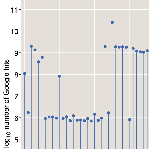
 5.675463855030418 

Huh? That sure doesn’t look like it’s converging to zero—not as \(\frac{1}{n!}\) or as \(\frac{n}{n - 1}\). As a matter of fact, it doesn’t look like it’s going to converge at all. The graph below suggests the sequence is made up of two alternating components, both of which appear to be slowly growing toward infinity as well as diverging from one another.

In trying to make sense of what we’re seeing here, it helps to change the output type of the div! function. Instead of applying the division operator /, which returns the quotient as a floating-point number, we can substitute the // operator, which returns an exact rational quotient, reduced to lowest terms.

div!(n)  =  n == 1 ? 1 : n // div!(n - 1)

Here’s the sequence of values for n in 1:20:

20-element Array{Real,1}:
       1      
      2//1    
      3//2    
      8//3    
     15//8    
     16//5    
     35//16   
    128//35   
    315//128  
    256//63   
    693//256  
   1024//231  
   3003//1024 
   2048//429  
   6435//2048 
  32768//6435 
 109395//32768
  65536//12155
 230945//65536
 262144//46189 

The list is full of curious patterns. It’s a double helix, with even numbers and odd numbers zigzagging in complementary strands. The even numbers are not just even; they are all powers of \(2\). Also, they appear in pairs—first in the numerator, then in the denominator—and their sequence is nondecreasing. But there are gaps; not all powers of \(2\) are present. The odd strand looks even more complicated, with various small prime factors flitting in and out of the numbers. (The primes have to be small—smaller than \(n\), anyway.)

This outcome took me by surprise. I had really expected to see a much tamer sequence, like those I worked out with pencil and paper. All those jagged, jitterbuggy ups and downs made no sense. Nor did the overall trend of unbounded growth in the ratio. How could you keep dividing and dividing, and wind up with bigger and bigger numbers?

At this point you may want to pause before reading on, and try to work out your own theory of where these zigzag numbers are coming from. If you need a hint, you can get a strong one—almost a spoiler—by looking up the sequence of numerators or the sequence of denominators in the Online Encyclopedia of Integer Sequences.

---

Here’s another hint. A small edit to the div! program completely transforms the output. Just flip the final clause, changing n // div!(n - 1) into div!(n - 1) // n.

div!(n)  =  n == 1 ? 1 : div!(n - 1) // n

Now the results look like this:

10-element Array{Real,1}:
  1                    
 1//2                  
 1//6                  
 1//24                 
 1//120                
 1//720                
 1//5040               
 1//40320              
 1//362880             
 1//3628800

This is the inverse factorial function we’ve already seen, the series of quotients generated when you march left to right through an ascending sequence of divisors \(1 \mathbin{/} 2 \mathbin{/} 3 \mathbin{/} \cdots \mathbin{/} n\).

It’s no surprise that flipping the final clause in the procedure alters the outcome. After all, we know that division is not commutative or associative. What’s not so easy to see is why the sequence of quotients generated by the original program takes that weird zigzag form. What mechanism is giving rise to those paired powers of 2 and the alternation of odd and even?

I have found that it’s easier to explain what’s going on in the zigzag sequence when I describe an iterative version of the procedure, rather than the recursive one. (This is an embarrassing admission for someone who has argued that recursive definitions are easier to reason about, but there you have it.) Here’s the program:

function div!_iter(n)
    q = 1
    for i in 1:n
        q = i // q
    end
    return q
end

I submit that this looping procedure is operationally identical to the recursive function, in the sense that if div!(n) and div!_iter(n) both return a result for some positive integer n, it will always be the same result. Here’s my evidence:

[div!(n) for n in 1:20]    [div!_iter(n) for n in 1:20]
            1                         1//1    
           2//1                       2//1    
           3//2                       3//2    
           8//3                       8//3    
          15//8                      15//8    
          16//5                      16//5    
          35//16                     35//16   
         128//35                    128//35   
         315//128                   315//128  
         256//63                    256//63   
         693//256                   693//256  
        1024//231                  1024//231  
        3003//1024                 3003//1024 
        2048//429                  2048//429  
        6435//2048                 6435//2048 
       32768//6435                32768//6435 
      109395//32768              109395//32768
       65536//12155               65536//12155
      230945//65536              230945//65536
      262144//46189              262144//46189

To understand the process that gives rise to these numbers, consider the successive values of the variables \(i\) and \(q\) each time the loop is executed. Initially, \(i\) and \(q\) are both set to \(1\); hence, after the first passage through the loop, the statement q = i // q gives \(q\) the value \(\frac{1}{1}\). Next time around, \(i = 2\) and \(q = \frac{1}{1}\), so \(q\)’s new value is \(\frac{2}{1}\). On the third iteration, \(i = 3\) and \(q = \frac{2}{1}\), yielding \(\frac{i}{q} \rightarrow \frac{3}{2}\). If this is still confusing, try thinking of \(\frac{i}{q}\) as \(i \times \frac{1}{q}\). The crucial observation is that on every passage through the loop, \(q\) is inverted, becoming \(\frac{1}{q}\).

If you unwind these operations, and look at the multiplications and divisions that go into each element of the series, a pattern emerges:

\[\frac{1}{1}, \quad \frac{2}{1}, \quad \frac{1 \cdot 3}{2}, \quad \frac{2 \cdot 4}{1 \cdot 3}, \quad \frac{1 \cdot 3 \cdot 5}{2 \cdot 4} \quad \frac{2 \cdot 4 \cdot 6}{1 \cdot 3 \cdot 5}\]

The general form is:

\[\frac{1 \cdot 3 \cdot 5 \cdot \cdots \cdot n}{2 \cdot 4 \cdot \cdots \cdot (n-1)} \quad (\text{odd } n) \qquad \frac{2 \cdot 4 \cdot 6 \cdot \cdots \cdot n}{1 \cdot 3 \cdot 5 \cdot \cdots \cdot (n-1)} \quad (\text{even } n).
\]

---

The functions \(1 \cdot 3 \cdot 5 \cdot \cdots \cdot n\) for odd \(n\) and \(2 \cdot 4 \cdot 6 \cdot \cdots \cdot n\) for even \(n\) have a name! They are known as double factorials, with the notation \(n!!\). Terrible terminology, no? Better to have named them “semi-factorials.” And if I didn’t know better, I would read \(n!!\) as “the factorial of the factorial.” The double factorial of n is defined as the product of n and all smaller positive integers of the same parity. Thus our peculiar sequence of zigzag quotients is simply \(\frac{n!!}{(n-1)!!}\).

A 2012 article by Henry W. Gould and Jocelyn Quaintance (behind a paywall, regrettably) surveys the applications of double factorials. They turn up more often than you might guess. In the middle of the 17th century John Wallis came up with this identity:

\[\frac{\pi}{2} = \frac{2 \cdot 2 \cdot 4 \cdot 4 \cdot 6 \cdot 6 \cdots}{1 \cdot 3 \cdot 3 \cdot 5 \cdot 5 \cdot 7 \cdots} = \lim_{n \rightarrow \infty} \frac{((2n)!!)^2}{(2n + 1)!!(2n - 1)!!}\]

An even weirder series, involving the cube of a quotient of double factorials, sums to \(\frac{2}{\pi}\). That one was discovered by (who else?) Srinivasa Ramanujan.

Gould and Quaintance also discuss the double factorial counterpart of binomial coefficients. The standard binomial coefficient is defined as:

\[\binom{n}{k} = \frac{n!}{k! (n-k)!}.\]

The double version is:

\[\left(\!\binom{n}{k}\!\right) = \frac{n!!}{k!! (n-k)!!}.\]

Note that our zigzag numbers fit this description and therefore qualify as double factorial binomial coefficients. Specifically, they are the numbers:

\[\left(\!\binom{n}{1}\!\right) = \left(\!\binom{n}{n - 1}\!\right) = \frac{n!!}{1!! (n-1)!!}.\]

The regular binomial \(\binom{n}{1}\) is not very interesting; it is simply equal to \(n\). But the doubled version \(\left(\!\binom{n}{1}\!\right)\), as we’ve seen, dances a livelier jig. And, unlike the single binomial, it is not always an integer. (The only integer values are \(1\) and \(2\).)

Seeing the zigzag numbers as ratios of double factorials explains quite a few of their properties, starting with the alternation of evens and odds. We can also see why all the even numbers in the sequence are powers of 2. Consider the case of \(n = 6\). The numerator of this fraction is \(2 \cdot 4 \cdot 6 = 48\), which acquires a factor of \(3\) from the \(6\). But the denominator is \(1 \cdot 3 \cdot 5 = 15\). The \(3\)s above and below cancel, leaving \(\frac{16}{5}\). Such cancelations will happen in every case. Whenever an odd factor \(m\) enters the even sequence, it must do so in the form \(2 \cdot m\), but at that point \(m\) itself must already be present in the odd sequence.

---

Is the sequence of zigzag numbers a reasonable answer to the question, “What happens when you divide instead of multiply in \(n!\)?” Or is the computer program that generates them just a buggy algorithm? My personal judgment is that \(\frac{1}{n!}\) is a more intuitive answer, but \(\frac{n!!}{(n - 1)!!}\) is more interesting.

Furthermore, the mere existence of the zigzag sequence broadens our horizons. As noted above, if you insist that the division algorithm must always chug along the list of \(n\) factors in order, at each stop dividing the number on the left by the number on the right, then there are only \(n\) possible outcomes, and they all look much alike. But the zigzag solution suggests wilder possibilities. We can formulate the task as follows. Take the set of factors \(\{1 \dots n\}\), select a subset, and invert all the elements of that subset; now multiply all the factors, both the inverted and the upright ones. If the inverted subset is empty, the result is the ordinary factorial \(n!\). If all of the factors are inverted, we get the inverse \(\frac{1}{n!}\). And if every second factor is inverted, starting with \(n - 1\), the result is an element of the zigzag sequence.

These are only a few among the many possible choices; in total there are \(2^n\) subsets of \(n\) items. For example, you might invert every number that is prime or a power of a prime \((2, 3, 4, 5, 7, 8, 9, 11, \dots)\). For small \(n\), the result jumps around but remains consistently less than \(1\):

If I were to continue this plot to larger \(n\), however, it would take off for the stratosphere. Prime powers get sparse farther out on the number line.

---

Here’s a question. We’ve seen factorial variants that go to zero as \(n\) goes to infinity, such as \(1/n!\). We’ve seen other variants grow without bound as \(n\) increases, including \(n!\) itself, and the zigzag numbers. Are there any versions of the factorial process that converge to a finite bound other than zero?

My first thought was this algorithm:

function greedy_balance(n)
    q = 1
    while n > 0
        q = q > 1 ? q /= n : q *= n
        n -= 1
    end
    return q
end

We loop through the integers from \(n\) down to \(1\), calculating the running product/quotient \(q\) as we go. At each step, if the current value of \(q\) is greater than \(1\), we divide by the next factor; otherwise, we multiply. This scheme implements a kind of feedback control or target-seeking behavior. If \(q\) gets too large, we reduce it; too small and we increase it. I conjectured that as \(n\) goes to infinity, \(q\) would settle into an ever-narrower range of values near \(1\).

Running the experiment gave me another surprise:

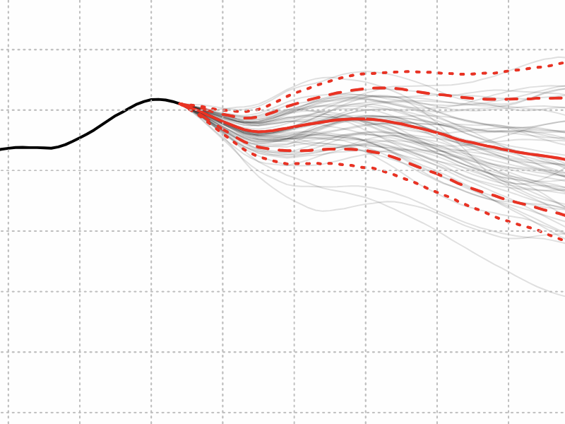
That sawtooth wave is not quite what I expected. One minor peculiarity is that the curve is not symmetric around \(1\); the excursions above have higher amplitude than those below. But this distortion is more visual than mathematical. Because \(q\) is a ratio, the distance from \(1\) to \(10\) is the same as the distance from \(1\) to \(\frac{1}{10}\), but it doesn’t look that way on a linear scale. The remedy is to plot the log of the ratio:

Now the graph is symmetric, or at least approximately so, centered on \(0\), which is the logarithm of \(1\). But a larger mystery remains. The sawtooth waveform is very regular, with a period of \(4\), and it shows no obvious signs of shrinking toward the expected limiting value of \(\log q = 0\). Numerical evidence suggests that as \(n\) goes to infinity the peaks of this curve converge on a value just above \(q = \frac{5}{3}\), and the troughs approach a value just below \(q = \frac{3}{5}\). (The corresponding base-\(10\) logarithms are roughly \(\pm0.222\). I have not worked out why this should be so. Perhaps someone will explain it to me.

The failure of this greedy algorithm doesn’t mean we can’t find a divisive factorial that converges to \(q = 1\). If we work with the logarithms of the factors, this procedure becomes an instance of a well-known compu­tational problem called the number partitioning problem. You are given a set of real numbers and asked to divide it into two sets whose sums are equal, or as close to equal as possible. It’s a certifiably hard problem, but it has also been called (PDF) “the easiest hard problem.”For any given \(n\), we might find that inverting some other subset of the factors gives a better approximation to \(n! = 1\). For small \(n\), we can solve the problem by brute force: Just look at all \(2^n\) subsets and pick the best one.

I have computed the optimal partitionings up to \(n = 30\), where there are a billion possibilities to choose from.

The graph is clearly flatlining. You could use the same method to force convergence to any other value between \(0\) and \(n!\).

And thus we have yet another answer to the question in the tweet that launched this adventure. What happens when you divide instead of multiply in n!? Anything you want.