Sunshine In = Earthshine Out

No computer simulations have ever had broader consequences for human life than the current generation of climate models. The models tell us that rising levels of atmospheric carbon dioxide and other greenhouse gases can trigger abrupt shifts in the planet’s climate; to avert those changes or mitigate their effects, the entire human population is urged to make fundamental economic and technological adjustments. In particular, we may have to forgo exploiting most of the world’s remaining reserves of fossil fuels. It’s not every day that the output of a computer program leads to a call for seven billion people to change their behavior.

Thus sayeth I in my latest American Scientist column (HTML, PDF). Climate is a subject I take up with a certain foreboding. The public “debate” over global warming has become so shrill and dysfunctional that I can barely force myself to pay attention, much less join the fray. As I worked on writing the column, I found myself tiptoeing through the polemical minefield, carefully avoiding any phrase that might be picked up by “the other side” and used against me. (“Even a writer for American Scientist has doubts about . . .”). When I handed in the text, my editors went over it with the same cautious anxiety—and they found a few places where they thought I hadn’t been careful enough.

This is not the kind of science I enjoy. I would much prefer to dwell in less-contentious corners of the cosmos, where I can play with my sticky spheres or my crinkly curves, and never give a thought to “the other side.” But now and then one must return to the home planet. Besides, the computer modeling that plays a major role in climate science is just my kind of thing.

So, for the past few months climate models have been my breakfast, lunch, and dinner, and my bedtime snack. I’ve been reading in the literature, and poring over source code; I’ve managed to get a couple of serious models running on a laptop. The American Scientist column says more about the rewards and frustrations of all these undertakings. Here I want to talk about a lighter side of the project: a little climate model of my own. The image below is just a static screen grab, but you can go play with the real thing if you’d like.

Okay, it’s not really all my own. The physics behind the model was explored more than 100 years ago by Svante Arrhenius. The first computer implementations were done by M. I. Budyko and William Sellers in 1969, and a third version was published by Stephen Schneider and Tevi Gal-Chen in 1973. But the JavaScript is mine. (Any mistakes are mine, too.)

The model is a simple one. The planet it describes is not the Earth we know and love but a bald sphere without continents or oceans, seasons or storms, or even day and night. Temperature is the only climatic variable. The globe is divided into latitudinal stripes five degrees wide, and temperatures are always uniform throughout a stripe. Other than warming and cooling, the only thing that can happen on this planet is freezing: If the temperature in a stripe falls below –10 degrees Celsius, it grows an ice sheet.

Why pay any attention to such a primitive model? Although a zillion details are missing, some important physical principles emerge with particular clarity. At the heart of the model is the concept of energy balance: If the Earth is to remain in thermal equilibrium with its surroundings, then it must radiate away as much energy as it receives from the Sun. The planet’s temperature will rise or fall in order to maintain this balance. The governing equation is:

\[Q (1 - \alpha) = \sigma T^{4}.\]

Here \(Q\) is the average intensity of incoming solar radiation in watts per square meter, \(\alpha\) is the albedo, or reflectivity, and \(T\) is temperature in Kelvins; \(\sigma\) is the Stefan-Boltzmann constant, which relates thermal emission to temperature. The numerical value of \(\sigma\) is \(5.67 \times 10^{-8} \mathrm{W m^{-2} K^{-4}}\). In other words, sunshine in = earthshine out.

If we know the solar input, we can calculate the Earth’s temperature at equilibrium by solving for \(T\):

\[T = \sqrt[4]{\frac{Q (1 - \alpha)}{\sigma}}\]

This is exactly what the energy-balance model does.

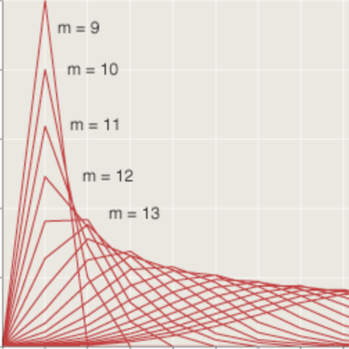
Two more effects need to be taken into account. First, most of the sun’s energy is received in the tropics, but it doesn’t all stay there. On the Earth, heat is redistributed by the process we call weather—evaporation and condensation, winds, storms, etc.—and also by ocean currents. In the model, the effect of all that swirly fluid dynamics is crudely approximated by a diffusive flow that simply smooths out temperature gradients.

Finally, there’s the greenhouse effect. Solar radiation at visible wavelengths passes through the Earth’s atmosphere to warm the surface, but the Earth emits at longer wavelengths, in the infrared; radiation in that part of the spectrum is absorbed by water vapor, carbon dioxide, and other minor constituents of the atmosphere. The blocked infrared emission raises the temperature at the surface by 30 degrees Celsius or more. The Earth would be a very chilly place without this effect, but the burning issue of the moment is how to avoid overheating. The model sidesteps all the complexities of atmospheric chemistry and absorption spectra; a single parameter, H, simply determines the fraction of outgoing radiation trapped by greenhouse gases.

The interface to the model has four controls—sliders that adjust the incident solar flux, the albedo of land, the albedo of ice-covered regions, and the greenhouse parameter. While playing with the slider settings, it’s not hard to get the model into a state from which there is no easy recovery. That’s what the reset button is for. (Too bad the real planet doesn’t have one.)

Some experiments you might try:

• The default greenhouse setting is H = 0.4, meaning that 40 percent of the outgoing radiation is intercepted. Lower the slider to below 0.2. The model enters a “snowball Earth” state, where ice sheets descend all the way to the Equator. Now return the greenhouse slider to the default setting of 0.4. The ice persists, and it will not melt away until the control is moved to a still higher setting. When the thaw does come, it is sudden and overshoots, leaving the planet in a much warmer state.
• Raise the greenhouse slider to about 0.45, where the polar ice cap disappears. Returning the slider to 0.4 does not restore the ice cap, and the polar areas remain several degrees warmer than they were before the greenhouse excursion.
• Raising the land albedo (so that more sunlight is reflected from snowfree surfaces, and less is absorbed) reveals another “ratchet” mechanism. Once the planet becomes totally icebound, further changes in the land albedo have no effect at all. The reason is simply that no ice-free land is exposed.
• Push the greenhouse slider toward the top of the scale. Beyond H = 0.75, tropical temperatures approach the boiling point of water, and the planet has obviously become uninhabitable. Question: What will happen at H = 1.0, where no radiation at all can escape the atmosphere?

Some of the extreme parameter values mentioned above yield fanciful results that would never be seen on the Earth. But certain interesting aspects of the model seem quite plausible. I am particularly intrigued by the presence of abrupt changes of state that look much like phase transitions. If we consider just the value of the greenhouse parameter H and the average global temperature T, we can draw a two-dimensional phase diagram in the (H, T) plane. The plot below traces the system’s trajectory as H is lowered from 0.4 to 0.2, then raised to 0.5, and finally returned to the initial setting of 0.4.

That four-sided loop is the hallmark of hysteresis (a term first introduced in the study of magnetic materials). Initially, as the greenhouse effect weakens, temperature falls off linearly. Then, at about H = 0.3, the curve steepens. (The stairsteps represent the freezing of successive zones of latitude.) Just below H = 0.218, the temperature falls off a cliff, dropping suddenly by 20 degrees Celsius. On the next segment of the curve, as H increases again, the temperature again responds linearly, but in a much colder regime. Only when H reaches 0.459 is warmth restored to the world, and this time there’s an abrupt upward jump of almost 35 degrees.

It’s no mystery what’s causing this behavior. There’s a strong feedback effect between cooling/freezing and warming/thawing. When the temperature in a latitude band falls below the –10 degree threshold, the zone ices over; the ice-covered surface is more reflective, and so less heat is absorbed, cooling the planet still more. Going in the other direction, when the ice melts, the exposed land absorbs more heat and brings still more warming.

The sharp, discontinuous transitions in the graph above could not happen on the real planet. They are possible in the model because it has no notion of heat capacity or latent heat; after every perturbation, the system instantly snaps back to equilibrium. But if the hysteresis loop in the model has unrealistically sharp corners, its basic shape is not impossible on a physical planet. What’s most important about the loop is that over a wide range of greenhouse parameters, the system has two stable states. At H = 0.4, for example, the world can have an average temperature of either 14 degrees of –22 degrees. That kind of bistability may well be possible in terrestrial climate.

Snowball Earth is not a fate we need to worry about anytime soon, but there is evidence that the planet actually went through such frozen states early in its history. The runaway greenhouse effect that would boil away the oceans is also not an immediate threat. So can we rest easy about living on a sedate, linear segment of the H-T curve? That’s a question that climate models are supposed to answer, but it’s beyond the scope of this particular model.