It’s tax time for Usaians. I’ve been plodding through the thick book of forms and instructions, tips and cautions, tables and worksheets and schedules and Paperwork Reduction Act notices. The unwelcome annual ritual always reminds me of the words of Hermann Weyl:
Our federal income tax law defines the tax y to be paid in terms of the income x; it does so in a clumsy enough way by pasting several linear functions together, each valid in another interval or bracket of income. An archeologist who, five thousand years from now, shall unearth some of our income tax returns together with relics of engineering works and mathematical books, will probably date them a couple of centuries earlier, certainly before Galileo and Vieta.
We should forgive Weyl his peevish tone; Form 1040 can put anyone in a grumpy mood. And maybe he had a point. The tax code has changed in many ways since Weyl gave his contemptuous assessment in 1940, but after all these years the income tax is still defined by a piecewise linear function. Here are the current rates for single taxpayers:
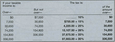
Graphically, the tax y as a function of taxable income x looks like this:

A few notes on this income-tax function:
- It is a proper function in the mathematical sense of that term: Every income x ≥ 0 is mapped to a unique tax y.
- The range of the function excludes negative incomes. In the real world, it’s quite possible to finish the year with a loss, but in tax land we are instructed: “Subtract line 42 from line 41. If line 42 is more than line 41, enter -0-.”
- The function touches the origin (zero income means zero tax) and is monotonically increasing. There is no income level where you can earn more money and pay less tax.
- The function is concave upward, which implies that the tax is progressive: People with higher incomes pay a higher proportion of their income as tax. But the progression stops at 35 percent: As x approaches infinity, the ratio y/x approaches a limiting value of 0.35.
- As a function defined by “pasting together” several straight-line segments, it is continuous but not differentiable at the points where the segments meet.
Weyl’s complaint against the tax code might have had something to do with the last of these observations—the jaggedness of the curve, or the discontinuity of the first derivative—but I don’t think that gets to the heart of the matter. No one really cares whether or not the tax curve is twice differentiable. What bothered Weyl, I suspect, was the mere fact that the tax function is defined as a concatenation of segments. He wanted a curve defined by a single expression that could be evaluated in the same way throughout the range of the function. (By the way, does this concept have a name, other than “not piecewise”? Should we call it a piecefoolish function?)
In setting out to create such a function, an obvious approach is fitting a polynomial to the half-dozen points given in the tax-rate table. But this process is not quite as easy and straightforward as it might seem. A major problem is that there are really seven points in the table rather than six. The 35-percent bracket continues indefinitely, extending to arbitrarily large incomes, and so there’s really an additional point on the curve, somewhere out there where x = ∞ and y = 0.35x. If you ignore this extra point, the 35-percent bracket disappears entirely. If you try to place the point at infinity, its influence on a least-squares fit will overwhelm all the other points. I don’t know a good solution to this problem, so I’ve adopted an arbitrary one. Noting that the lengths of the tax brackets are roughly in geometric proportion, I’ve placed a seventh point at a position that maintains this approximate relation, x = 750,000, y = 242,360.50.
Let’s begin with a linear (i.e., first-degree) polynomial model of the tax brackets. Some people call this a “flat tax,” although that term seems to me more appropriate for a scheme in which everyone pays the same amount of tax; here, it means everyone pays at the same rate, or the same proportion of income. In any case, I don’t think the flat-tax fans would be enthusiastic about this flat tax:
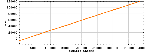
Following this formula, everyone with a taxable income below about $19,000 pays a negative tax, or in other words receives a subsidy from the government. For those with zero income, the subsidy is more than $6,000. Meanwhile, all those above the $19,000 threshold pay 32.6 percent of their income as tax.
A quadratic fit to the tax-table data looks slightly less inflamatory:
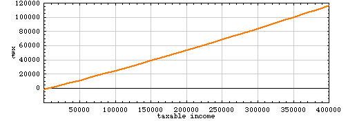
There’s still a bit of negative income tax, but it doesn’t kick in until income falls below $9,500, and the maximum subsidy is about $2,500. Overall, the curve is really quite a close fit to the data, with an r2 value of 0.9995. The largest residual error between the fitted curve and the data is $2,484, at the zero-income point. Perhaps one could use these linear and quadratic approximations to the tax-rate data to argue that the shape of the tax function “wants” to include a negative tax for the lowest incomes, but the official curve has been artificially cut off to prevent this. (The Earned Income Credit does allow some low-income taxpayers to have an effective negative tax, but the structure of the credit is different from that of the models discussed here. The EIC provides almost no benefit at zero income; the maximum negative tax is at an income of between $6,000 and $16,000.)
We can match the data points in the tax table as closely as we please simply by going to higher-degree polynomials, but this is not necessarily a good idea. A sixth-degree polynomial will thread itself through all seven of the specified points:

In between the specified points, the curve has some suspicious-looking lumps and sags. People earning about $250,000 seem to be getting a break, and those with incomes of $350,000 are paying a penalty. On taking a step back and looking at a broader range of incomes, the curve turns out to be far more bizarre:
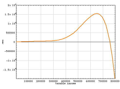
This is a tax function that Vice President Cheney might well appreciate. The Cheney family has reported that they had taxable income of $1.6 million last year; according to the sixth-degree polynomial, they should be due a refund—a negative income tax—of a little over $2 billion. Meanwhile, poor George W. Bush, who reported a meagre $642,905 of taxable income, is unlucky enough to find himself near the peak of that big hump in the curve. He would be asked to pay a tax of more than $1.5 million—almost three times his total earnings.
So maybe fitting a curve to the existing tax structure is not such a good idea after all. Let’s try to construct a curve that’s similar in overall form to the present tax brackets but not so rigidly constrained by the data in the table. The curve in the graph below is a quadratic that passes through three of the bracket-defining points, {0, 0}, {30650, 4220} and {336550, 97653}:

Over the range of incomes shown, the shape of the curve is a reasonable match (at least by eye) to the piecewise tax function of the Internal Revenue Service. By construction, the function yields a zero tax for zero income and is positive everywhere else. It is concave upward. But there’s still a big problem:
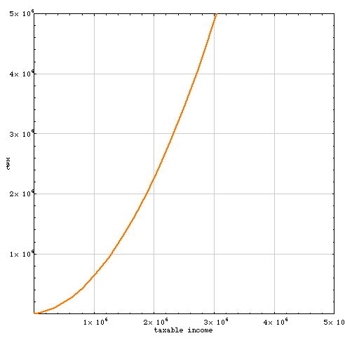
The quadratic curve was constructed from data in the range between zero and a few hundred thousand dollars; outside that range, the function is free to go wild. In this case the slope of the curve becomes greater than 1 at about x = $1.8 million; beyond that income level, the tax rate is greater than 100 percent, so that the tax owed exceeds earnings. Even those of us who ardently want to soak the rich will have to admit that collecting such taxes might be difficult.
It begins to seem that Weyl’s request for a simple tax function is not so easy to satisfy. We can have a piecewise definition and make it do anything we want, but that is what Weyl was trying to get away from. We can have a flat tax, given by a first-degree polynomial, but many people think that would be socially and economically undesireable. With a polynomial of any degree higher than 1, the tax will eventually diverge either to +∞ or –∞.
On the other hand, we have certainly not exhausted the list of candidate functions. How about this one: y = x – x1–ε, where ε is some positive number less than 1? Here’s what the tax curve looks like for ε = 0.027.

This is a fairly good match to the existing tax function over the range of x shown, and it doesn’t blow up at larger values of x. As x goes to infinity, y/x very slowly approaches 1 from below. (The tax rate reaches 90 percent for incomes above about 1037 dollars.) The function is concave upward, and it’s positive for all positive x.
In this formula the expression x1–ε could be replaced by any slowly growing function of x. An appealing candidate is log(x), but getting a sensible tax curve out of a logarithmic function is a bit of a chore. The first problem appears at the origin: log(x) diverges to negative infinity as x approaches zero from above, and so a small income will earn you an arbitrarily large negative tax. We can avoid the problem by working with log(x+1). A further difficulty is that log(x) grows so very slowly that over any wide range of incomes, y = x – log(x) doesn’t differ appreciably from y = x. The closest I’ve been able to come to an acceptable tax function is 0.335 x – 973 log(x + 1) + 1578:
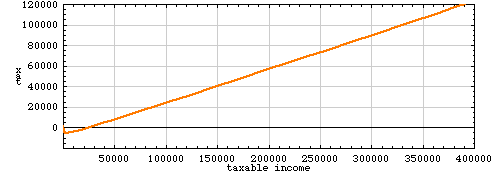
Here the tax is negative for any income below about $25,000.
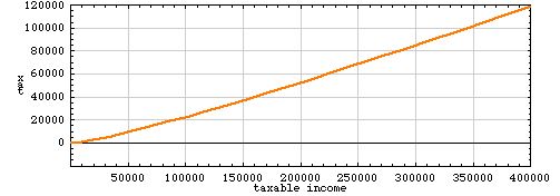
The function x – x/log(x), shown below, is somewhat better-behaved, although again fudge factors are needed to avoid singularities near the origin. (The actual equation being graphed here is –7.706(x+1)/log(x+2) + 0.893x – 2.297.)
The mention of x/log(x) leads to a further thought, and a final fantasy. The function x/log(x) is well known as an approximation to pi(x), the function that counts the number of primes less than x. I think Weyl might have been pleased if the instructions to Form 1040 required you to enumerate the prime numbers up to your income level. This innovation would at last bring the federal tax code out of the age of Galileo and Viete, all the way up to Gauss and Riemann.