Only Correlate!
by Brian Hayes
Published 28 May 2011
I’m not actually a shill for Google Labs, although it may seem that way from all my recent (and ongoing) attention to the Google Ngram Viewer: four posts (1, 2, 3, 4) and an American Scientist column, so far. What I particularly like about Google Labs is that they share their toys. They create Big Data projects that everybody can play with. For those of us without a server farm on the back 40, that’s a rare opportunity.
The latest Labs release is Google Correlate. If you have a time series—data expressed as a function of date, for any subinterval of the period since 2003—Correlate will try to identify Google search queries that exhibit a similar temporal pattern of activity. All this is easier to understand with an example. For a specimen time series, consider the interest-rate index known as the 1-year CMT, which is published every week. I scraped seven years of CMT data from this web site, and uploaded the file to Correlate. I got back a list of 100 phrases whose popularity as Google search terms has followed a trajectory more or less similar to that of the interest rates. As it happens, none of those highly correlated terms has an obvious connection to financial affairs. Roughly half of them are related to cell phones (“cingular” and “treo” turn up over and over). But the term with the strongest correlation (r=0.9751) is the phrase “pill identification”:

In other words, the gradual rise in interest rates during the early 2000s was paralleled by a steady growth in the number of people seeking help in identifying the contents of mysterious unlabeled vials in the medicine cabinet. Then, sometime in 2007, both trends reversed direction. Why should these particular variables be so closely correlated? If there is a reason, I have no idea what it is. And I must immediately insert the obligatory disclaimer: Correlation is not causation. Emphatically so in this case. If you are trying to predict the future course of interest rates, I do not recommend tracking popular interest in pill identification. Or vice versa.
At a more personal level, there’s a time series I have been tracking since 2007: the volume of spam arriving in my email inbox. My records are monthly, whereas Google Correlate wants weekly data, so I did some resampling and smoothing, and came up with this:

The best match, shown in the graph, is the mildly enigmatic query “ashford blackboard login.” Many of the other correlated series suggest a seasonal theme that I can understand in retrospect but that I did not see coming before looking at the results: “honda accord 2009,” “celica 2009,” “rav4 2009,” “2009 altima coupe,” “new cars 2009,” “2009 ranger,” etc. The most distinctive features of the spam curve are a peak in the fall of 2008, a deep dip the following winter, and an even stronger surge in the summer of 2009. Evidently shoppers for cars in the 2009 model year followed a similar trend line. (But again I would caution that spam volume is unlikely to be a good predictor of automobile sales.)
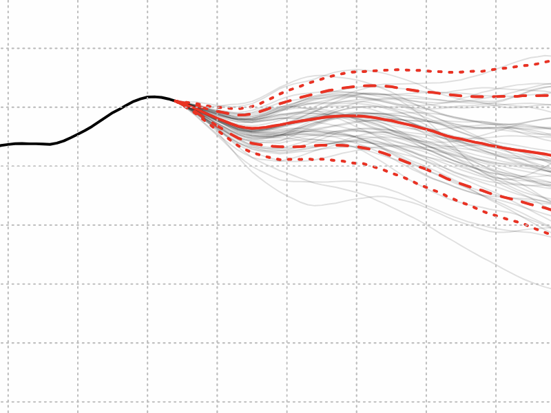
These results might be taken to suggest that every conceivable time series must be correlated with some set of Google queries, however farfetched the association. I tried submitting a few random walks, covering the same time span as the spam series, and they too fetched up matching queries from the Google database:

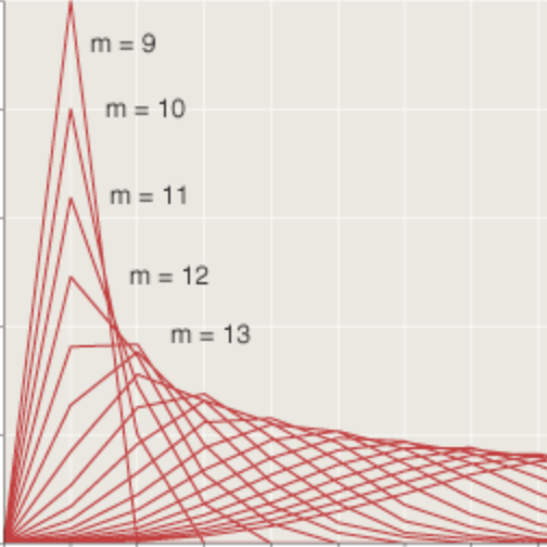
At the opposite end of the spectrum from a random walk, I tried some rigidly artificial probes, such as a series with nonzero entries only in the month of May. Sure enough, there are search-engine queries that follow the same recurrent annual pattern:

A time series that has all of its energy concentrated in a single pulse elicits from the database a variety of flash-in-the-pan topics—queries that came and went and were never heard of again.

Without too much work we could enumerate all such one-month wonders.
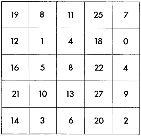
It is not the case, however, that every possible time series has a close correlate somewhere in the Google collection. Here is an example of a series for which Correlate finds no query that matches closely enough to bother reporting:

This is a weekly record of miles driven in the family car. Should we be surprised that not a single series among the tens of millions of queries in the Google database comes close to matching this pattern? One approach to this question is to ask just how many series of this kind might exist. The mileage record covers 364 weeks. As a lower bound, suppose the mileage associated with each week could have just two possible values: either we drove the car or we didn’t, so the mileage is either zero or greater than zero. Then there are 2364 (or about 10110) possible time series—many orders of magnitude greater than the total number of Google searches since the company was founded. Thus the set of queries in the Google archive must be an extremely sparse subset of all possible time series. Most of the series we could construct would necessarily come up empty. (I note in passing that there’s interesting structure in that mileage log of mine, which I never knew about until I graphed it—but that’s a story for another day.)
A really interesting question is how Google Correlate does it. Even with “only” tens of millions of queries in the database, comparing a submitted series with all the candidates would be impossibly expensive. A white paper explains:
In our Approximate Nearest Neighbor (ANN) system, we achieve a good balance of precision and speed by using a two-pass hash-based system. In the first pass, we compute an approximate distance from the target series to a hash of each series in our database. In the second pass, we compute the exact distance function on the top results returned from the first pass.
Thus the basic strategy is precomputation: Spend a lot of time in advance computing a succinct signature or hash associated with each time series in the database; then quickly compare hash values when looking to match a submitted time series.
A few further miscellaneous notes:
Google Correlate evolved from earlier work on tracking influenza outbreaks by monitoring search-engine queries. Initially this required a batch computation lasting hours, even when run on hundreds of computers. The new hash-based search takes less than a second. (Algorithms and data structures still count for more than hardware.)
Google Correlate includes a geographic component alongside the temporal database. If you have data distributed over the 50 U.S. states, you can retrieve Google queries that exhibit a similar spatial pattern. (I have not experimented with this system.)
Even if you don’t have a time series or a geographic data set of your own, you can play with the new service by cross-correlating one search query against others. For example, enter the term “solstice” in the search box, and you’ll see a graph with exactly the pattern of twice-a-year spikes that you might expect. You also get a list of other search terms whose temporal pattern has similar features. One of those correlated terms is “italian seafood salad.” A glance at the corresponding graph suggests there’s only half a correlation in this case:

I didn’t know until just a few minutes ago that frutti di mare was a dish to be eaten at the winter solstice.
Responses from readers:
Please note: The bit-player website is no longer equipped to accept and publish comments from readers, but the author is still eager to hear from you. Send comments, criticism, compliments, or corrections to brian@bit-player.org.
Publication history
First publication: 28 May 2011
Converted to Eleventy framework: 22 April 2025

Google is all about precomputation.
My favorite example of correlation-not-causation: A table showing the correlation between smoking and lung cancer on a country-by-country basis in a certain scientific magazine was followed, some months later, by a letter to the editor containing a similar table, showing the country-by-country correlation between smoking and cholera. The more smoking, the less cholera.
I had a few minutes of fun searching for times of the day (5 AM, 11 AM, 2 PM, 4PM…) and then for angle measures (60 degrees, 75 degrees, 90 degrees, 105 degrees…). It appears that when someone needs a calculator, everybody needs it!
This is quite interesting. Surely you can use this to analyze various things, I’m especially thinking it can be useful when doing marketing.
Hi,
Thanks for the great post. I don’t come from a math background but rather a marketing background. Alot of my real world data is on a monthly basis. I noticed in your post that so was your and that you were able to smooth it out to provide weekly data. How do you go about doing that?
Thanks!
@Chris:
I first converted from monthly to daily data, dividing each monthly total by the number of days in that month. Then it’s easy to create weekly tallies by summing up successive seven-day periods.
In the monthly-to-daily conversion, you may have to deal with leap-year issues—the bane of all calendrical calculations. But weeks are sweet; every one of them has exactly seven days.
You might also want to do some smoothing of the daily counts, using a moving-window average. (That is to say, you replace each daily value by the average—which might be a weighted average—of that value and the k preceding and following values.) In my case I found that smoothing did not have a large effect on the results.
Well, I’ve never seen anybody eating frutti di mare on winter solstice in Italy. I think you would even have trouble finding them in the supermarket in december.