Googling the lexicon

In 1860, when work began on the New English Dictionary on Historical Principles (better known today as the Oxford English Dictionary), the basic plan was to build an index to all of English literature. Volunteer readers would pore over texts and send in paper slips with transcribed quotations, each slip showing a word in its native context. The slips of paper were collected in a “scriptorium,” where they were sorted alphabetically and became the raw material for the work of the lexi­cographers. The project was supposed to be completed in 10 years, but it took almost 70. Some 2,000 readers contributed 5 million quo­tation slips, citing phrases from 4,500 published works.

Google and Harvard have now given us a new index to the corpus of written English—and they’ve thrown in a few other languages as well. The data cover more than 500 billion word occurrences, drawn from 5,195,769 books (estimated to be 4 percent of all the books ever printed). The entire archive is being made available for download into your home scriptorium, under a Creative Commons license.

The project was announced December 16th with the online release of a paper to appear in Science. Here’s a quick rundown:

Publication: The Science article is “Quantitative Analysis of Culture Using Millions of Digitized Books.” It is supposed to remain freely available to nonsubscribers. See also the supplementary online material.

Authors: Jean-Baptiste Michel and Erez Lieberman Aiden of Harvard, with a dozen co-authors: Yuan Kui Shen, Aviva P. Aiden, Adrian Veres, Matthew K. Gray, The Google Books Team, Joseph P. Pickett, Dale Hoiberg, Dan Clancy, Peter Norvig, Jon Orwant, Steven Pinker and Martin A. Nowak.

Languages: English, Chinese, French, German, Russian and Spanish. There are actually five archives for English, based on various subsets and intersecting sets of the underlying texts (e.g., British vs. U.S.).

Data format: The OED quotations were meaningful hunks of text—typically a sentence. Here we get n-grams. A 1-gram is a single word or other lexical unit, such as a number. An n-gram is a sequence of n consecutive 1-grams. The Harvard-Google collaboration has compiled lists of n-grams for values of n between 1 and 5. Thus the 1-gram files are lists of single words, and the other files give snippets of text consisting of two, three, four or five words. For each n-gram we learn the number of occurrences per year from 1550 through 2008 as well as the number of pages on which the n-gram is found and the number of books in which it appears.

Links to related stuff:

• The Harvard group’s “Culturomics” web site.
• The download page for the data sets.
• An n-gram viewer from Google Labs.
• An earlier (2006) release of Google n-gram data. (The 2006 n-grams were from the web, rather than from books.)

Links to less-related stuff:

• Wordnet, a lexical database developed by George A. Miller of Princeton.
• My American Scientist article on Wordnet.
• Linguistic Data Consortium (lots more word data).

•     •     •

If you want to play with this new toy, the place to begin is the Google n-gram viewer. At this site you submit a query to an online copy of the database and get back a graph showing normalized n-gram frequencies for a selected range of years. Here’s a search on the days of the week. (The graphs from the n-gram viewer are very wide, and bit-player is very skinny. I’ve squeezed the graphs horizontally; hover on them to unsqueeze. (See nifty effect in Safari, Chrome, maybe other Webkit browsers.))

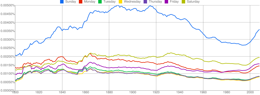
The results are not surprising, I think, but they’re interesting. “Sunday” is an outlier. “Monday” was once the next-most-often-mentioned day, but around 1860 it was overtaken by Saturday, and now it has also fallen behind Friday. As for the middle of the week—nobody cares about those days.

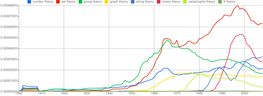
Here is a collection of “theory” bigrams: “number theory”, “set theory”, “group theory”, “graph theory”, “string theory”, “chaos theory”, “catastrophe theory”, “K theory”. Which of them had the highest frequency in the 20th century? (I guessed wrong.)

(By the way, the graph above has a strange lump in the first decade of the 20th century. I think it’s a metadata error. The same anomalous blip turns up for many other search terms, such as “transistor” and “Internet”. Somewhere along the way, a batch of books from 2005 were recorded as having been published in 1905. (Geoff Nunberg at Language Log has pointed out many other problems with Google Books metadata.))

Here are a few magazines I have written for.

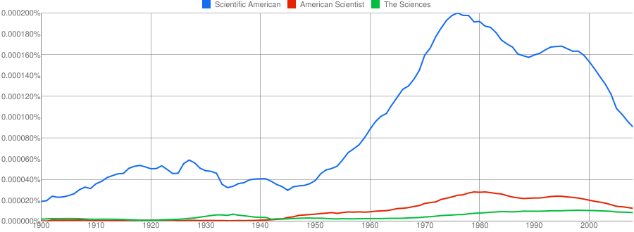
I’m afraid there’s a dismal pattern in this data: Publications reach their peak and begin declining soon after I arrive. (But the most recent plunge at Scientific American is not my doing.)

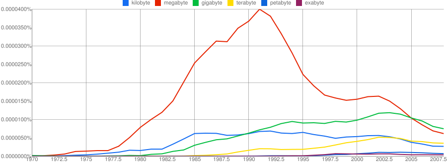
The graph below offers some tech trends. It appears we have officially entered the age of the gigabyte, and terabytes are coming on strong:

Next is a list of rare (even nonexistent) words: “uroboros”, “widdershins”, “abacot”, “baragouin”, “funambulist”, “futhark”, “gongorism”, “hapax legomenon”, “hypnopompic”:

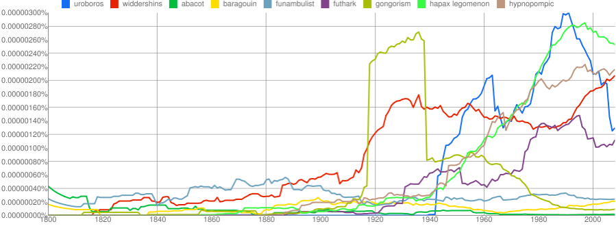
It’s curious that so many of these archaic-looking terms seem to be increasing in frequency.

At the other end of the spectrum are some very common words:

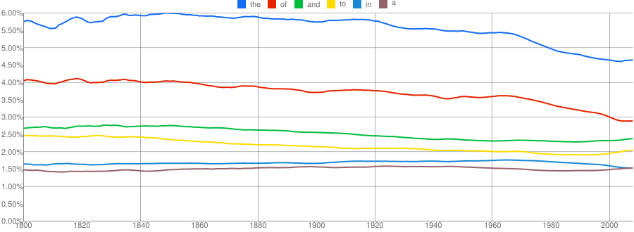
Again there’s a mild surprise here: The ordering of these words in the Google Books corpus apparently differs from that of the list usually cited.

•     •     •

I think the n-gram browser is great fun, but it provides access to only one aspect of the data set: We can plot the normalized frequency of specific n-grams as a function of time. There are many other kinds of questions one might ask about all these words. For starters, I’d like to invert the query function and find all n-grams that have a given frequency. (An obvious project is to compile a list of the commonest words and phrases in the corpus.)

At an even more elementary level: What is the distribution of word lengths in English?

Here’s another question: In the formula “I [verb] you”, what are the commonest verbs? The information needed to answer this question is present in the 3-gram files, but the Google viewer does not provide a means to get at it.

With appropriate software, the n-grams could also be used for language synthesis—generating highly plausible generic gibberish through a Markov process.

Still another idea is to explore the history of spelling errors and typos over the centuries. Did the introduction of the qwerty keyboard lead to different kinds of errors? How about the later introduction of spell-checking software, and the concomitant decline of proofreading as a trade?

Furthermore, the n-gram files are full of numbers as well as words. Can we learn anything of economic interest by charting the prevalence of numbers that look like monetary amounts? (It’s easy to search for specific strings of digits, such as “$9.99″, but I would like to treat these values as numbers rather than sequences of digits, so that “0.99″, “.99″ and “0.99000″ would all be numerically equal.)

The way to carry out any of these projects is to download the full n-gram files and start writing software to explore them. I’ve taken my first step in that direction: I’ve bought a new disk drive to hold the data. Next I’m going to borrow a faster Internet connection to do the bulk of the downloading. After that, I must confess that I don’t have a lot of confidence about how best to proceed. The scale of these data sets is roughly a terabyte, which in this age of Big Data is no more than a warmup exercise. But it’s bigger than anything I’ve ever tried to grab hold of personally. I’ll be grateful for advice from those with more experience.

The n-gram lists come in fragments. The 1-grams, for example, are broken up into 10 files, each of which weighs about a gigabyte. Within each file the n-grams are listed alphabetically, but the distribution across files is random. (For example, file 0 has “gab”, “gaw” and “gay”, but “gag”, “gap” and “gas” are elsewhere.) Ordinarily, my first impulse would be to run a big merge-sort over these files, putting all the words in order. But maybe that’s exactly the wrong thing to do; keeping them scattered is a potential opportunity for multithread parallelism.

Even casual browsing through the raw n-gram files is quite a revelation. They really are raw. Word frequencies are the prototypical example of a Zipf distribution, which has notoriously long tails. It follows that when you choose an entry at random from one of the n-gram files, you are likely to be waaaaaaay out in the aberrant fringe, looking at symbol strings that you might or might not recognize as English words. Here are 20 lines selected at random from a 1-gram file:

1-GRAM          YEAR   COUNT   PAGES   BOOKS 
lilywhites      1994       1       1       1
Carneri         2002      24      24      12
Thurh           1971       1       1       1
Elsee           1832       5       5       4
cFMte           2008      12      12      12
COFFEE          1876     288     270     167
APO3            1990       6       3       1
Odumbara        1963      15      15       6
connubialibus   1967       1       1       1
Pickerel        1900      65      54      34
fubje&ed        1757       6       6       5
nader           1971      34      29      19
fiyled          1782       1       1       1
existfed        1993       2       2       2
Soveit          2007       1       1       1
monongahela     1939       4       4       4
suffeiing       1851       6       6       6
brake           1774      12      10       7
ofBrasenose     1951       3       3       3
Horas           1798       3       3       2

This is a pretty strange stew. There are obscure words, several proper names and abbreviations, as well as quite a few misspellings and nonstandard capitalizations. But the oddities that stand out most sharply have another origin: They are errors of optical character recognition. A word that was correct in the original document has gotten all fubje&ed up in the course of scanning. Of the 20 items listed above, 5 appear to be marred by OCR errors, so this is not just a matter of minor contamination. My best guess is that the word recorded as “fubje&ed” appeared in the 1757 book as:

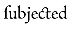
with an initial long “s” that was assimilated to an “f” and a “ct” ligature that the OCR program confused with an ampersand.

The files are rife with such problems. Another case that caught my eye was “quicro”. As a Scrabble player, I ought to know that 18-point word! It turns out to be an OCR error for the Spanish verb “quiero”. And why is there a Spanish word in an English lexicon? Well, when I ran a search at Google Books, the top hit for “quicro” was Robert Southey’s Commonplace Book, published in 1850, which is properly classified as an English work even though it includes many long passages of Spanish and Portuguese verse.

Should we worry about such distractions? The real “quiero” is roughly 200 times as frequent as “quicro”, so the OCR error will not have a major statistical impact. Perhaps the most disturbing effect of the OCR noise is that it greatly lengthens the already-long tail of the frequency distribution. Suppose a word appears 100,000 times in the corpus. If the OCR process is 99.9 percent accurate, 100 instances of the word will be read incorrectly; in the worst case, each erroneous reading could be different, adding 100 spurious entries to the lexicon.

Cleaning up this mess looks like a major undertaking. (If it were easy, Google would have done it already.)

The long tail of the distribution has already been truncated to some extent: No n-gram is included in the data set unless it appears at least 40 times in the corpus of texts. For many kinds of analysis, an even higher threshold might be appropriate—excluding all terms that fall below 400 or maybe even 4,000 occurrences. But that still won’t eliminate all the OCR errors: “quickfilver” appears 5,411 times.

•     •     •

Before I go, I want to tell one more story, which is a mystery story. It all began when I was trying out a few seasonal phrases:

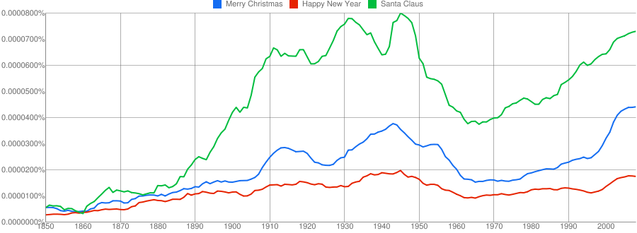
Note the distinctive and dramatic dip in all three frequencies starting in the late 40s or early 50s and continuing into the 70s, with an eventual strong recovery in the 90s. The frequencies fall by roughly 50 percent, then return to the neighborhood of their earlier peak. What’s going on here? Did the Grinch steal Christmas, and then give it back? Was there a backlash against Jingle Bells in the era of disco dancing and Watergate?

As a check on these results I tried a few terms associated with other holidays, unrelated to the midwinter madness. The same pattern emerged:

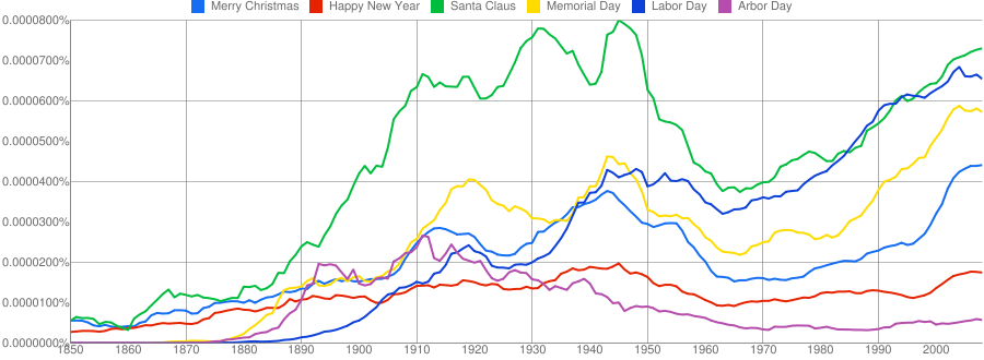
As a further control, I added still more phrases, this time with no obvious connection to any holiday whatever. All that the terms have in common is that they fall into roughly the same range of frequencies:

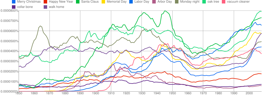
The slump in the 60s and 70s is still visible in this augmented set of words. The dip looks rather like one of those episodes of mass extinction in the fossil record. And it provokes the same question: What caused it? And what ended it?

Of course not all words and phrases follow this pattern. Because the curves represent normalized frequencies—the count of each n-gram’s occurrences divided by the total number of all n-gram occurrences—a valley in any one n-gram’s frequency must be balanced by a peak for some other word or words. This fact leads to a hypothesis about the cause of the Great Postwar Santa Depression. The 50s and 60s were a period in which technical and scientific publishing bloomed, thereby diluting the share of printed books that would be likely to mention phrases such as “Santa Claus” and “vacuum cleaner”; instead we got volumes full of “asymptotic freedom”, “chymotrypsin inhibitor” and “field-effect transistor”.

The trouble with this notion is that the explosive growth of the sci/tech vocabulary did not end in the 1980s or 90s; thus it’s hard to understand how Santa has made such a spectacular comeback.

Here’s one wild guess at an explanation. Most of the books that Google has scanned come from university libraries, and so I wonder if we might be observing an artifact of the acquisition and retention policies of university librarians. Suppose that libraries tend to buy a broad cross-section of newly published titles, but when shelf space gets scarce, the half-life of Quantum Information Theory is longer than that of Frosty the Snowman. As a result of this selective culling, Santa books from the 60s have melted away, but those from the 90s have not yet disappeared. Could such practices account for the dip and the recovery? If you have a better idea, please share.