
I often use a computer to create graphics, but there was a time when I used graphics to compute. That era came back to me the other day in the library. I was browsing among dusty volumes in the folio section when I came upon this:
The Design of Diagrams
for Engineering Formulas
and
The Theory of Nomography
by
Laurence I. Hewes, B. Sc., Ph. D.
and
Herbert L. Seward, Ph. B., M. E.
McGraw-Hill Book Company, Inc.
1923
The clerk at the circulation desk observed that there was no record anyone had ever borrowed this book. Although the records don’t go all the way back to 1923, I wouldn’t be surprised if I’m the first reader of this volume in 30 or 40 years.
It’s a book full of nomograms and similar graphic devices, with instructions on how to create them. Here’s a simple example for calculating the volume of a torus:
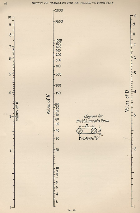
If you know any two of d, V and D, you can find the third quantity by laying a straightedge across the scales. (Quick quiz: What’s that constant in the formula V = 2.4674d2D?)
I used to see computational aids like this all the time. Some magazine I read in the seventies (I’m not sure which one—maybe Electronics?) published a new nomogram every month. But now such diagrams have a decidedly fusty look. They’re like tools you might find in an old blacksmith shop or a tannery; it’s a challenge just to figure out how they worked and what they were used for. You find yourself admiring the workers who created useful products with such implements.
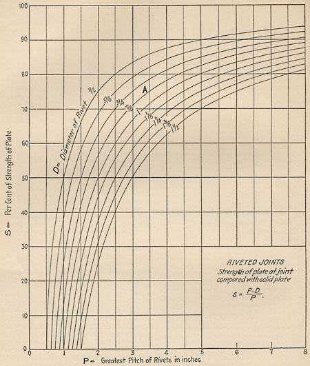
The graphic device below is for calculating the strength of a metal plate pierced by rivet holes:
Did the engineers who specified the half-inch gusset plates for certain joints on the I-35W bridge in Minneapolis rely on such aids? The preliminary report from the National Transportation Safety Board (.pdf) doesn’t comment on the computational methods that might have been used when the bridge was designed in the early 1960s. In any case, it’s not at all obvious which is more error-prone—pencil and paper, slide rule, nomogram, CAD software.
The Theory of Nomography—as Hewes and Seward term their art—could hardly be more distant from modern computing practice. For one thing, it converts arithmetic into geometry; nowadays, we’re more likely to go the opposite way. A nomogram also emphasizes a static, declarative style of representing knowledge: A single diagram embodies all the relations of several variables, and one method solves for any unknown. Most digital computing is procedural rather than declarative; the emphasis is on step-by-step algorithms to go from givens to answers.
I’m not about to give up silicon in favor of paper computers, but I do find some of these diagrams both beautiful and illuminating. Here’s a nomogram for solving the quadratic equation z2+pz+q=0:
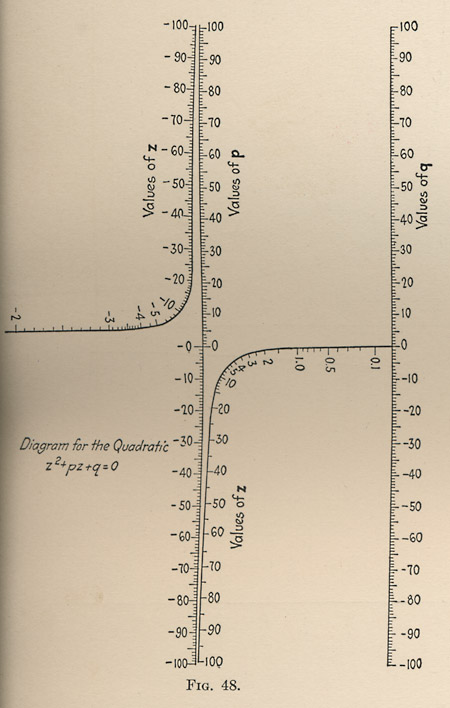
Instead of three straight-line scales, as in the formula for the volume of a torus, we have two linear scales and a hyperbola. A moment’s thought reveals why the diagram must have this form: For any combination of the coefficients p and q, the equation must have either two roots or no (real) root. One branch of the hyperbola carries all the positive roots and the other all the negative values of z. Poking around in the diagram brings various properties of the equation into sharp focus. For example, if you lay a straightedge across the diagram in such a way that it passes through the point p=0, then it will either cut the two branches of the hyperbola symmetrically (if q is negative) or it will miss both branches (if q is positive). This is no surprise—the roots of z2+q=0 had better be plus and minus the square root of q—but the graphic presentation carries a lot of explanatory force.
Hewes and Seward give an even more elaborate tableau for solving a cubic equation:
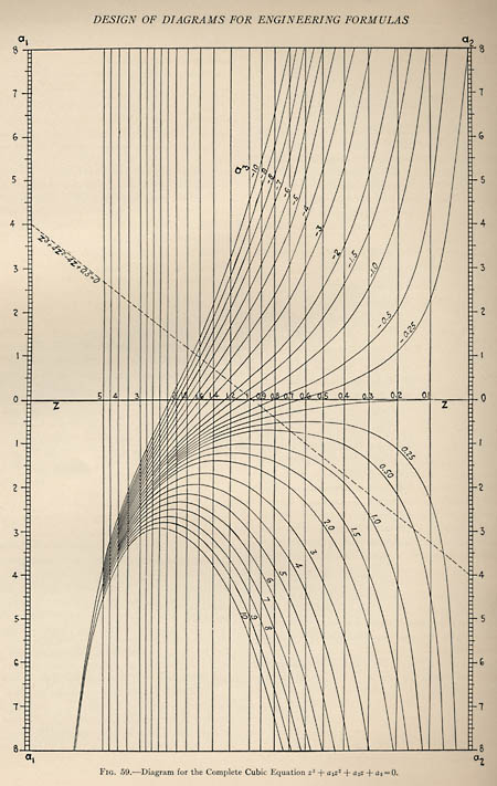
The dashed line drawn across this diagram represents a straightedge placed so as to solve the particular instance z3+4z2-4z+0.5=0. The straightedge is set to the points 4 and –4 on the left and right scales, and then the roots are read off by projecting vertically from the intersections of this line with the curve labeled 0.50. Working by eye, the roots appear to lie at about 0.15 and 0.7. Newton’s method—the archetype of iterative, step-by-step computations—gives 0.14758497342482376768480 and 0.69902089681305967783231. (On the SAGE server at the University of Washington, finding each of those roots took a couple of hundredths of a second.)
Note: Ask Dr. Math has an informative article on nomograms (or nomographs) with lots of references. One of the references led me to a 1999 lecture by Thomas Hankins, published in Isis (Hankins, Thomas L. 1999. Blood, dirt, and nomograms: A particular history of graphs. Isis 90(1):50–80). Hankins traces the origin and early history of the nomogram, which I had never known. Both the name and the concept came from Maurice d’Ocagne of the École des Ponts et Chaussées in Paris toward the end of the 19th century. Their first uses were in calculations needed for railroad construction.
Update 2008-03-05: Ron Doerfler, in a blog called Dead Reckonings, has several illuminating and thorough essays on the construction of nomographs, including a very fishy example laid out on an elliptic curve. The rest of the blog is also worth reading. Thanks to Mitch Burrill for the pointer.
What makes you think the curve in the nomogram for the quadratic equation is a hyperbola?
What makes you think it’s not? What are the alternatives?
I’m curious how you got those roots, since only about half the digits are correct. More-precise values (with all digits correct) for the three roots of this polynomial are: -4.84660587023924317159898089597, 0.147584973426213536603410049667, and 0.699020896813029634995570846304.
(As a Sage developer, I’m particularly curious, because if Sage gave you those wrong answers then that’s a bug I want to fix.)
@ Carl Witty: When you pointed out the error, my first thought was that I must have been too lax in setting the tolerance of the algorithm, or something equally careless. But apparently that’s not the problem.
The root-finder code comes from here: https://www.sagenb.org/home/pub/1500
And here is how I defined the polynomial we’re trying to evaluate:
f(x) = x^3 + 4*x^2 - 4*x + 0.5
I’m still very much a Sage neophyte, and it took me a little while to sniff out what’s wrong with that definition. The root-finder code returns correct results for *this* polynomial:
f(x) = x^3 + 4*x^2 - 4*x + 1/2
So it appears we have a simple case of inaccuracy introduced by floating-point truncation. What I don’t understand, though, is that Sage tells me (0.5==1/2) returns True.
As I said, I’m a Sage newbie, so enlightenment is welcome!
Cool stuff.
I had almost the same questions a few months ago…
The Sage coercion rules (for doing arithmetic and comparisons between values of different types) include the following:
1) In operations between different types, if one type is more precise than the other, the more precise value is coerced to the less precise type and then the operation is performed at the less precise type. (This is similar to the rules for significant figures I learned in school.)
2) Floating-point literals default to 53-bit precision (the precision of an IEEE double-precision floating-point value) (unless the floating-point literal is specified with many digits; then it uses enough bits to account for all the given digits).
This root-finder tries to do everything in 80-bit precision, but it is “poisoned” by the 53-bit “0.5″. So most of the arithmetic is actually done with 53-bit precision, which explains your inaccurate results.
The above rules also explain (0.5 == 1/2); the infinitely-precise 1/2 is coerced to a floating-point 0.5, and then the comparison says that the two values are equal.
These rules give results that are sometimes counter-intuitive (as you’ve seen), but usually they work well, and we haven’t been able to come up with better rules.
I don’t want to make trouble, and I know I’m in over my head, but….
If 0.5 and 1/2 aren’t truly equal–if you can’t substitute one for the other in all contexts–is it a good idea for (0.5 == 1/2) to claim they are equivalent?
More important, why *aren’t* they equal? In 53 bits or any other floating-point representation, 0.5 and 1/2 both have an exact binary representation, namely 0.100….
I’ve just looked around at the way a few other systems deal with this issue. In both Common Lisp and Scheme (my home turf), (= 1/2 0.5) is true, but (= 1/10 0.1) is false (because decimal 1/10 has no exact finite representation in binary). In Mathematica, both of the corresponding expressions are true, which is also the case in Sage; these systems are evidently smart enough to figure out that the two notations refer to the same number. The difference is that Mathematica seems to be more consistent about treating the quantities as equals. Solving our little cubic equation in Mathematica gives the same (correct) result whether the constant term is expressed as 0.5 or 1/2.
What’s going on in Sage that 0.5 and 1/2 are the same when I run a direct comparison but they behave differently in the context of the Newton’s method algorithm?
Let me add one final point: It’s just this sort of difficulty that makes me grateful I don’t design highway bridges, or anything else that lives depend on.
I’m a beginner at this computer algebra stuff; I just happen to know a little bit about Sage (and a lot about this part of Sage).
I don’t know if it’s a good idea that (0.5 == 1/2) when they don’t act the same. I am pretty sure that it’s a good idea that (2 == 4/2), even though they don’t act exactly the same (in Sage, 2 is of type Integer, and 4/2 is of type Rational).
I do think it makes sense that multiplying floating-point numbers of different precisions should give a result of the lesser precision, and that multiplying a floating-point number by an integer should give a floating-point number of the same precision as the input. I suppose an argument could be made for using a more complicated rule in the case of addition (if you have 1000 as a 10-bit float, and 1 as a 1-bit float, then it could make sense that their sum would be 1001 as a 10-bit float); but using the same rule for addition and multiplication makes things a lot simpler.
Mathematica actually seems to have roughly similar rules to Sage, based on the following experiments:
sage: n(pi, digits=30) + 1/2
3.64159265358979323846264338328
sage: n(pi, digits=30) + 0.5
3.64159265358979
In[1]:= N[Pi, 30] + 1/2
Out[1]= 3.64159265358979323846264338328
In[2]:= N[Pi, 30] + 0.5
Out[2]= 3.64159
We see that Mathematica defaults to using many fewer bits for the literal 0.5, but both systems treat 0.5 as being a limited-precision float, and 1/2 (in this context) as being essentially infinite precision.
Based on this experiment, I’m guessing that if you wrote the equivalent Newton’s method code in Mathematica, you would get essentially the same result as in Sage, where a 0.5 would make the whole computation less precise.
If you invoke an explicit polynomial root-finder in Sage, then you do get the same results whether you use 0.5 or 1/2; this is because it coerces the coefficients to high precision floats at the start.
sage: z = polygen(RR)
sage: (z^3 + 4*z^2 - 4*z + 0.5).roots(ring=RealField(100))
[(-4.8466058702392431715989808960, 1),
(0.14758497342621353660341004967, 1),
(0.69902089681302963499557084630, 1)]
sage: (z^3 + 4*z^2 - 4*z + 1/2).roots(ring=RealField(100))
[(-4.8466058702392431715989808960, 1),
(0.14758497342621353660341004967, 1),
(0.69902089681302963499557084630, 1)]
“What makes you think it’s not?”
What makes you think I think it’s not?
@ Carl Witty: I don’t pretend to know what the Right Thing is. But if 0.5 is such a suspect value that you have to deliberately discard a bunch of perfectly good digits when you evaluate n(pi, digits=30) + 0.5, then I don’t see how to justify the declaration 1/2==0.5.
Of course there’s also the irony that all this disputation began with a graphic device that provides an accuracy of no more than two decimal places. I’m sure Hewes and Seward would have been quite impressed by a method that gives an answer that begins to drift away from exactness in the 12th decimal place.
@ Barry Cipra: I know the curve must be a hyperbola because the book says it is, and any high school student can tell you that the book is never wrong. Here’s the passage in Hewes and Seward (with inconsequential reformatting):
“The equation of the three scales may for convenience be written as follows: x = –z/(1+z), y = –z^2/(1+z) ; x = –1, y = p ; x = 0, y = q. The scale for z is then graduated on an hyperbola with the asymptote x = –1. Figure 48 is the diagram. No scale factors are used but the unit on the horizontal axis is taken 100 times that on the vertical axis, as this convenient device is always available. The roots are read at the points where the straight line through the given values of p and q on their respective scales, cuts this hyperbola graduated with z.”
I renew my question: If we look at this curve and assume it has some reasonably concise mathematical definition, what could it be other than a hyperbola? I can’t think of another plausible candidate, but perhaps I’m missing something obvious.
We’re clearly both wrong in thinking it is (or isn’t) a hyperbola, since Hewes and Seward say it’s *an* hyperbola….
My underlying point, if I have one, is that while it’s relatively easy to see how the logarithmic scales on the three lines and the fact that the V line is twice as far from the D line as it is from the d line come from the formula for the volume of the torus (by the way, 2.4674 is a good approximation to (355/226)^2….), and obvious that the curves for the riveted joints are hyperbolae, it’s not at all obvious, to me at least, how and why the last two nomograms work. I had to derive the parameterization you quoted from Hewes and Seward. (I did so before my initial post, so I actually did know the curve to be a hyperbola. It’s worth noting that the equation is
y = 1-x-1/(1+x)
so in particular, the hyperbola does not have a horizontal asymptote — it curves back down to the right of the q-line and back up to the left of the point corresponding to z=-2.) As for the cubic-equation nomogram, can you tell (without looking it up!) what family of curves is being used?
On a quasi-related matter, I’ve always wondered how well drawn these old diagrams are. Having scanned them into your computer, you should be able to superimpose properly scaled computer-generated versions of the same curves, using appropriate equations (e.g., the parameterizations x=-z/(1+z), y=-z^2/(1+z), etc.) to see if the draftsman’s drawing departs visibly from computer’s presumably correct rendition. Some discrepancies could, of course, be due to distortions created in the scanning procedure, but even that would be of interest.