In 1877 the German mathematician Georg Cantor made a shocking discovery. He found that a two-dimensional surface contains no more points than a one-dimensional line.
Thus begins my latest column in American Scientist, now available in HTML or PDF. The leading actor in this story is the Hilbert curve, which illustrates Cantor’s shocking discovery by leaping out of the one-dimensional universe and filling up a two-dimensional area. David Hilbert discovered this trick in 1891, building on earlier work by Giuseppe Peano. The curve is not smooth, but it’s continuous—you can draw it without ever lifting the pencil from the paper—and when elaborated to all its infinite glory it touches every point in a square.
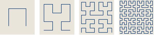
Above: The first through fourth stages in the construction of the Hilbert curve. To generate the complete space-filling curve, just keep going this way.
To supplement the new column I’ve built two interactive illustrations. The first one animates the geometric construction of the Hilbert curve, showing how four copies of the generation-n curve can be shrunken, twirled, flipped and reconnected to produce generation n+1. The second illustration is a sort of graphic calculator for exploring the mapping between one-dimensional and two-dimensional spaces. For any point t on the unit line segment [0, 1], the calculator identifies the corresponding point x, y in the unit square [0, 1]2. The inverse mapping is also implemented, although it’s not one-to-one. A point x, y in the square can correspond to multiple points t on the segment; the calculator shows only one of the possibilities.
The Hilbert-curve illustrations are posted in the Extras department here at bit-player.org. I encourage you to go play with them, but please come back and read on. I have some unsolved problems.
I built the Hilbert mapping calculator in part to satisfy my own curiosity. It’s fine to know that every point t can be matched with a point x, y, but which points go together, exactly? For example, what point in the square corresponds to the midpoint of the segment? The answer in this case is not hard to work out: The middle of the segment maps to the middle of the square: (t = 1/2) → (x = 1/2, y = 1/2). Shown below are a few more salient points, as plotted by the calculator:

Rational points of the form t = n/12, for integer 0 ≤ n ≤ 12, are mapped into the unit square according to their positions along the Hilbert curve. For example, t = 3/12 = 1/4 is mapped to the point x = 0, y = 1/2, at the midpoint of the square’s left edge. Note that the Hilbert curve drawn in the background of the illustration is a fifth-stage approximation to the true curve, but the positions of the colored dots are calculated to much higher precision.
Looking at this tableau led me to wonder what other values of t correspond to “interesting” x, y positions. In particular, which fractions along the t segment project to points on the perimeter of the square? Which t values go to points along one of the midlines, either vertical or horizontal? To narrow these questions a little further, let’s just consider fractions whose denominator is a prime. (In all that follows I ignore fractions with denominator 1, or in other words the end points of the t segment.)
The diagram above already reveals that fractions with denominator 2 and 3 are members of the “interesting” class. The value t = 1/2 maps to the intersection of the two midlines. And t = 1/4, 1/3, 2/3 and 3/4 all generate x, y points that lie on the perimeter. Can we find interesting fractions with other prime factors in the denominator? Yes indeed! Here is the Hilbert mapping for fractions of the form n/5:

Hilbert mapping for fifths. In the calculator you can generate this output by entering */5 into the input area labeled “t =”. It turns out that (t = 2/5) → (x = 1/3, y = 1), and (t = 3/5) → (x = 2/3, y = 1).
Note that 2/5 and 3/5 map to points on the upper boundary of the square. By a simple sequential search I soon stumbled upon two more “interesting” examples, namely n/13, and then n/17.

Hilbert mapping for t = 0/13, 1/13, 2/13 … 13/13. The fractions t = 3/13, 4/13, 9/13 and 10/13 yield x, y coordinates on the perimeter of the square.

Hilbert mapping for 17ths. The fractions t = 1/17, 4/17, 6/17 and 7/17 correspond to points on the perimeter, as well as the mirror images of these points when reflected through the vertical midline.
At this point I began to think that prime-denominator fractions yielding perimeter points must be lying around everywhere just waiting for me to gather them up. And I was not surprised by their seeming abundance. After all, there are infinitely many points on the perimeter of the square, and so there must be infinitely many corresponding t values—even if we confine our attention to the rational numbers.
When I continued the search, however, my luck ran out. In the “t=” box of the calculator I typed in all fractions of the form */p for primes p < 100; I found no points on the perimeter other than the ones I already knew about, namely those for p = 3, 5, 13 and 17.
So I automated the search. It turns out the next prime denominator yielding perimeter points is 257. Typing */257 into the calculator produces this garish display:

Points of the form t = n/257. There are 32 points that lie along the perimeter of the square.
Beyond 257 comes an even longer barren stretch. Surveying all prime denominators less than 10,000 failed to reveal any more that produce Hilbert-curve perimeter points.
The obvious next step is to look at larger Fermat numbers, but there’s a complication. Fermat’s claim that all such numbers are prime turned out to be overreaching a little bit; beyond the first five, every Fermat number checked so far has turned out to be composite. Still, we can see if they give us Hilbert perimeter points. The sixth Fermat number is 4294967297, and sure enough there are fractions with this number in the denominator that land on the perimeter of the Hilbert curve. For example, t = 4/4294967297 converges to x = 0, y = 1/32768. We can also check the factors of this number (which have been known since 17291732, when Euler identified them as 641 and 6700417). With a bit of effort I pinned down a few fractions with 6700417 in the denominator, such as 2181/6700417, that are on the perimeter.
It’s the same story with the seventh Fermat number, 18446744073709551617. Both this number and its largest prime factor, 67280421310721, yield perimeter points. I have not looked beyond the seventh F number. Would I be as reckless as Fermat if I were to conjecture that all such numbers generate Hilbert-curve perimeter points?
Thus the known prime denominators that give rise to perimeter points are the five Fermat primes, 3, 5, 17, 257 and 65537, as well as two prime factors of larger Fermat numbers, 6700417 and 67280421310721. Oh, and 13. I almost forgot 13. Who let him in?
Of course there are many (infinitely many) perimeter points whose associated t values do not have a prime denominator. If we run through all fractions whose denominator is less than 1,000 (when reduced to lowest terms), this is the set of denominators that maps to perimeter points:
{3, 4, 5, 12, 13, 16, 17, 20, 48, 51, 52, 63, 64, 65, 68, 80, 192, 204, 205, 208, 252, 255, 256, 257, 260, 272, 273, 320, 341, 768, 771, 816, 819, 820, 832}
It’s another curious bunch of numbers, with patterns that are hard to fathom. (The OEIS is no help.) I thought at first that the numbers might be composed exclusively of the primes I had identified earlier (as well as 2). This notion held together until I got to 63, which of course has a factor of 7. Then I thought a slightly weaker condition might hold: Other factors are allowed, but at least one factor must be drawn from the favored set. That lasted until I reached 341, which factors as 11 × 31. There must be some logic behind the selection of these numbers, but the rule escapes me. One more peculiarity: Every even power of 2 appears, but none of the odd powers.
Here is the analogous set of denominators for t values that project to the two midlines of the Hilbert curve:
{2, 4, 6, 10, 12, 16, 20, 26, 34, 48, 52, 64, 68, 80, 102, 126, 130, 192, 204, 208, 252, 256, 260, 272, 320, 410, 510, 514, 546, 682, 768, 816, 820, 832}
One difference jumps out immediately: All of these numbers are even. Yet the sets have more than half their elements in common. Every even member of the perimeter set is also a member of the midline set. Also note that again only even powers 2 are included (apart from 2 itself).
I doubt that any deep mathematical truth hinges on the question of which numbers correspond to perimeter points on the Hilbert curve. Nevertheless, having allowed myself to get sucked into this murky business, I would really like to come out of it with some glimmer of understanding. So far that eludes me.
I can explain part of what’s happening here by looking more closely at the mechanism of the mapping from t to x, y. The process is easiest to follow if t is expressed as a quaternary fraction (i.e., base 4). Thus we view t as a list of “quadits,” digits drawn from the set {0, 1, 2, 3}. Each stage of the mapping process takes a single quadit and uses it to choose one of four affine transformations to apply to the current x, y coordinates, from H0 to H3.
\[ \mathbf{H}_0 =
\left(
\begin{matrix}
0 & 1/2\\
1/2 & 0
\end{matrix}
\right)
\left(
\begin{matrix}
x\\
y
\end{matrix}
\right)
+
\left(
\begin{matrix}
0\\
0
\end{matrix}
\right)
\qquad
\mathbf{H}_1 =
\left(
\begin{matrix}
1/2 & 0\\
0 & 1/2
\end{matrix}
\right)
\left(
\begin{matrix}
x\\
y
\end{matrix}
\right)
+
\left(
\begin{matrix}
0\\
1/2
\end{matrix}
\right)
\]
\[ \mathbf{H}_2 =
\left(
\begin{matrix}
1/2 & 0\\
0 & 1/2
\end{matrix}
\right)
\left(
\begin{matrix}
x\\
y
\end{matrix}
\right)
+
\left(
\begin{matrix}
1/2\\[0.3em]
1/2
\end{matrix}
\right)
\qquad
\mathbf{H}_3 =
\left(
\begin{matrix}
0 & -1/2\\
-1/2 & 0
\end{matrix}
\right)
\left(
\begin{matrix}
x\\
y
\end{matrix}
\right)
+
\left(
\begin{matrix}
1\\
1/2
\end{matrix}
\right)
\]
The sequence of quadits determines a sequence of transformations, which in turn determines the mapping from t to x, y. Here is the Javascript that implements the mapping function in the online Hilbert-curve calculator:
function hilbertMap(quadits) {
  var pt, t, x, y;
  if ( quadits.length === 0 ) {
    return new Point(1/2, 1/2);   // center of the square
  }
  else {
    t = quadits.shift();          // get first quadit
    pt = hilbertMap(quadits);     // recursive call
    x = pt.x;
    y = pt.y;
    switch(t) {
      case 0:     // southwest, with a twist
        return new Point(y * 1/2 + 0, x * 1/2 + 0);
      case 1:     // northwest
        return new Point(x * 1/2 + 0, y * 1/2 + 1/2);
      case 2:     // northeast
        return new Point(x * 1/2 + 1/2, y * 1/2 + 1/2);
      case 3:     // southeast, with twist & flip
        return new Point(y * -1/2 + 1, x * -1/2 + 1/2);
    }
  }
}
If you’re not in a mood to pick your way through either the linear algebra or the source code, I can give a rough idea of what’s going on. With each 0 quadit, the x, y point drifts toward the southwest corner of the square. A 1 quadit steers the point toward the northwest, and likewise a 2 quadit nudges the point to the northeast and a 3 quadit to the southeast. From these facts alone you can predict the outcome of simple cases. An uninterrupted string of 0 quadits has to converge on the southwest corner of the square, which is just what’s observed for t = 0. In the same way, a quadit sequence of all 1s has to end up in the northwest corner. What t value corresponds to (0.1111111…)4? This is the quaternary expansion of 1/3, which explains why we see (t = 1/3) → (x = 0, y = 1).
The quaternary expansion of 2/5 is (0.121212…)4. Let’s trace what the Javascript code above does when it is given a finite prefix of this number. In the illustration below, the prefix is just four quadits, (0.1212)4. 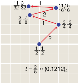 The recursive procedure effectively works back-to-front through the sequence of quadits. The x and y coordinates are given initial values of 1/2 (in the middle of the square). The first transformation is H2, which amounts to x → (y/2 + 1/2), y → (x/2 + 1/2); after this operation, the position of the x, y point is (3/4, 3/4). The next quadit is 1, and so the H1 transformation is applied to the new x, y coordinates. H1 specifies x → (x/2), y → (y/2 + 1/2); as a result, the point moves to (3/8, 7/8). Another round of H2 followed by H1 brings the position to (11/32, 31/32). Generalizing to a more precise calculation with a longer string of quadits, it’s easy to see that the nth location in this progression will have a y coordinate equal to \(\frac{2^{n}-1}{2^{n}}\); as n goes to infinity, this expression converges to 1.
Here the quaternary expansion of 2/5 is compared with the expansions of a few other fractions that correspond to y = 1 perimeter points:
t = 2/5 = (0.12121212…)4 → (x = 1/3, y = 1)
t = 6/17 = (0.11221122…)4 → (x = 1/5, y = 1)
t = 22/65 = (0.11122211…)4 → (x = 1/9, y = 1)
t = 86/257 = (0.11112222…)4 → (x = 1/17, y = 1)
Every number t whose quaternary expansion consists exclusively of 1s and 2s projects to some point along the northern boundary of the square. It would be satisfyingly tidy if we could make an analogous statement about the other three boundary edges. For example, if all 1s and 2s head north, then quadits made up of 0s and 3s ought to wind up on the southern edge. But it’s not so simple. Consider these cases:
t = 1/17 = (0.00330033…)4 → (x = 1/5, y = 0)
t = 4/17 = (0.03300330…)4 → (x = 0, y = 2/5)
t = 13/17 = (0.30033003…)4 → (x = 1, y = 2/5)
t = 16/17 = (0.33003300…)4 → (x = 4/5, y = 0)
The behavior of 1/17 and 16/17 is what you might expect: They go south. But 4/17 and 13/17 migrate not to the bottom of the square but to the two sides. If strings of 1s and 2s are so well-behaved, what’s the matter with strings of 0s and 3s? Well, the geometric transformations associated with quadrants 1 and 2 are simple scalings and translations. The matrices for quadrants 0 and 3 are more complicated: They introduce rotations and reflections. As a result it’s not so easy to predict the trajectory of an x, y point from the sequence of quadits in the t value. In any case I have not yet found a simple and obvious general rule.
The case of t = n/13 is no less perplexing:
t = 1/13 = (0.010323010323…)4 → (x = 1/3, y = 0)
t = 4/13 = (0.103230103230…)4 → (x = 0, y = 2/3)
t = 9/13 = (0.230103230103…)4 → (x = 1, y = 2/3)
t = 12/13 = (0.323010323010…)4 → (x = 2/3, y = 0)
When I trace through these transformations, as I did above for t = 2/5, I get the right answer in the end, but I haven’t a clue to the logic that drives the trajectory. I certainly can’t look at such a sequence of quadits and predict where the point will wind up.
I am left with more questions than answers. Furthermore, I don’t know whether the questions are genuinely difficult or if I am just missing something obvious. (It wouldn’t be the first time.) Anyway, here are the two big ones:
- Can we prove that all Fermat numbers give rise to Hilbert-curve perimeter points? And, for composite Fermat numbers, will we always find that at least one of the factors shares this property?
- Apart from the Fermat primes and factors of composite Fermat numbers, is 13 the only “sporadic” case? If so, what’s so special about 13?
I lack the mental muscle to answer these questions. Maybe someone else will make progress.
Update 2013-04-27: After publishing this story yesterday, I extended my search for “interesting” prime denominators, covering the territory between 257 and 65537. I found one new specimen: 61681. Twenty t values with this denominator yield perimeter points on the Hilbert curve. The smallest of them is t = 907/61681 → (x = 0, y = 101/1025). The repeating unit of the quaternary expansion of this fraction is (0.00033003223330033011)4.
Update 2013-04-29: Please see the comments! Several readers have provided illuminating insights, including a finite-state machine by ShreevatsaR that recognizes the class of quaternary-digit sequences that map to the perimeter of the square. And, as a further result of ShreevatsaR’s analysis, we have yet another “interesting” prime denominator: 15790321.