The National Research Council is getting ready to release a new assessment of graduate-education programs in the U.S. The previous study, published in 1995, gave each Ph.D.-granting department a numerical score between 0 and 5, then listed all the programs in each discipline in rank order. For example, here’s the top-10 list for doctoral programs in mathematics (as presented by H. J. Newton of Texas A&M University):
 rank    school                 score
    1    Princeton               4.94
    2    Cal Berkeley            4.94
    3    MIT                     4.92
    4    Harvard                 4.90
    5    Chicago                 4.69
    6    Stanford                4.68
    7    Yale                    4.55
    8    NYU                     4.49
    9    Michigan                4.23
   10    Columbia                4.23
Note that the scores of the first two schools are identical (to two decimal places), and the first four scores differ by less than 1 percent. Given the uncertainties in the data, it seems reasonable to suppose that the ranking could have turned out differently. If the whole survey had been repeated, the first few schools might have appeared in a different order. Doctoral candidates in mathematics are presumably sophisticated enough to understand this point. Nevertheless, the spot at top of the list still carries undeniable prestige, even when you know that the distinction could be merely an artifact of statistical noise.
The committee appointed by the NRC to conduct the new graduate-school study wants to avoid this “spurious precision problem.” They’ve adopted some jazzy statistical methods—mainly a technique called resampling—to model the uncertainty in the data, and they’ve also decreed that the results will be presented differently. There will be no sorted master list showing overall ranks in descending order. Instead the programs in each discipline will be listed alphabetically, and each program will be given a range of possible ranks. For example, a program might be estimated to rank between fifth place and ninth place. Let’s call such a range of ranks a rank-interval, and denote it {5, 6, 7, 8, 9} or {5–9}.
For a hypothetical set of 10 institutions, A through J, here’s what a set of rank-intervals might look like.
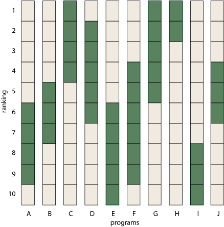
Acknowledging the uncertainty in your findings is commendable. But let’s be realistic. If you actually want to make use of these results—for example, if you’re a student choosing a grad-school program—the first thing you’re going to do is sort those bars into some sort of rank order, trying to figure out which school is best and how they all stack up against one another. In other words, you’re going to undo all the elaborate efforts the NRC committee has put into obscuring that information.
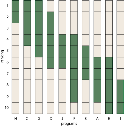
Below is one possible ordering of the bars. I have sorted first on the top of the rank-intervals, then, if two columns have the same top rank, I’ve sorted on the bottom rank. Other sorting rules give similar but not identical results. For example, sorting on the midpoints of the intervals would interchange columns B and F.
Question 1. Does sorting a set of rank-intervals by one of these simple rules yield a consistent and meaningful total ordering of the data? To put it another way, can you trust this attempt to reconstruct a ranking?
I hasten to add that this is not really a practical question about finding the best grad school. If you’re facing such a choice in real life, the NRC rank-intervals are not the only available source of information. But, for the sake of the mathematical puzzle, let’s pretend that all we know about schools A through J is embodied in those ranges of rankings.
It turns out that rank-intervals have some fairly peculiar behavior. Ranges of ratings are not a problem. If the NRC merely gave each school a fuzzy rating on the 0-to-5 scale, no one would have much trouble interpreting the results. But when you turn fuzzy ratings into fuzzy rankings, there are hidden constraints. For example, not all sets of rank-intervals are well-formed.
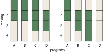
The set at left is impossible because there’s no one in last place. (We can’t all be above average.) The example at right is also nonsensical because D has no ranking at all. For a set of rank-intervals to be valid, there has to be at least one entry in each row and each column.
That’s a necessary condition, but not a sufficient one, as the two graphs below illustrate.
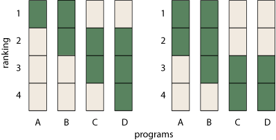
Do you see the problem with the example at left? Column B has a rank-interval of {1–2}, but in fact B can never rank first because A has no alternative to being first. The case at right is conceptually similar but a little subtler: If B is ranked third, then either first place or second place will have to remain vacant.
The underlying issue here is the presence of constraints or linkages within a set of rankings. Suppose you have calculated ratings and rankings of several schools, and then some new information turns up about one school. You can change the rating of that school without any need to adjust other ratings, but not so the ranking. If a school goes from third place to fourth place, the old fourth-place school has to move to some other rung of the ladder, and somebody has to fill the vacancy in third place. These interdependencies are obvious in a non-fuzzy ranking, but they also exist in the fuzzy case. You can’t just assign arbitrary rank-intervals to the items in a set and assume they’ll all fit together. This observation leads to a second question:
Question 2. What are the admissible sets of rank-intervals? How do we characterize them?
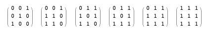
I have a partial answer to this question. It goes like this. Any ranking of k things must be a permutation of the integers from 1 through k. A permutation can be embodied in a permutation matrix—a square k × k matrix in which every row has a single 1, every column has a single 1, and all the other entries are 0. For example, here are the six possible 3 × 3 permutation matrices:
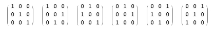
They correspond to the rankings (1, 2, 3), (1, 3, 2), (2, 1, 3), (3, 1, 2), (2, 3, 1) and (3, 2, 1).
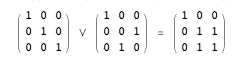
Since a permutation matrix represents a specific (non-fuzzy) ranking, we can build up a set of rank-intervals by taking the OR-sum of two or more permutation matrices. What do I mean by an OR-sum? It’s just the element-by-element sum of the matrices using the boolean OR operator, ∨, instead of ordinary addition. OR has the following addition table:
                      0 ∨ 0 = 0
                      0 ∨ 1 = 1
                      1 ∨ 0 = 1
                      1 ∨ 1 = 1
For the first two 3 × 3 matrices shown above the arithmetic sum is:
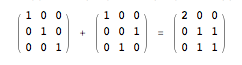
whereas the OR-sum looks like this:
Every valid set of rank-intervals must correspond to an OR-sum of permutation matrices, simply because a set of rank-intervals is in fact a collection of permutations. The converse also holds: Any OR-sum of permutation matrices yields an admissible set of rank-intervals. Thus the OR-sums of permutation matrices—let’s call them ormats for brevity—are in one-to-one correspondence with the admissible sets of rank-intervals. (There’s just one catch when applying this idea to the NRC study. The columns of an ormat may well have “gaps,” as in the column pattern (0 1 1 0 0 1 1), which corresponds to the rank-interval {2–3, 6–7}. Will the NRC allow such discontinuous ranges in their grad-school assessments? Perhaps the issue will never come up in practice. In any case, I’m ignoring it here.)
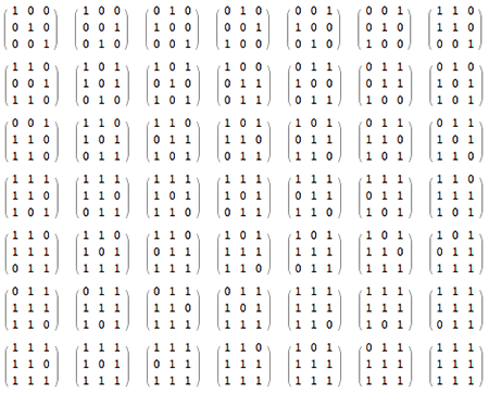
Arithmetic sums of permutation matrices form an open-ended, infinite series; in contrast, there are only finitely many distinguishable OR-sums. The reason is easy to see: Ormats have k2 entries, each of which can take on only two possible values, and so there can’t be more than \(2^{k^{2}}\) distinct matrices. Because of the various constraints on the arrangement of the entries, the actual number of ormats is smaller. For example, at k = 3 the \(2^{k^{2}}\) upper bound allows for 512 ormats, but there are only 49:
Thus we come to the next question.
Question 3. For each k ≥ 1, how many distinct ormats can we build by OR-ing subsets of k × k permutation matrices? Is there a closed-form expression for this number?
I have answers only for puny values of k.
   k       upper bound        # of ormats
   1                 1                  1
   2                16                  3
   3               512                 49
   4            65,536              7,443
   5        33,554,432          6,092,721
   6    68,719,476,736                  ?
The tallies of ormats were calculated by direct enumeration, which is not a promising approach for larger k. (I note—to spare folks the bother of looking—that the sequence 1, 3, 49, 7443, 6092721 does not yet appear in the OEIS.)
To extend this series, we might try to exploit the internal structure and symmetries of the ormats. By sorting the columns and rows of the matrices, we can reduce the 49 3×3 ormats to just six equivalence classes, with the following exemplars:
Enumerating just these reduced sets of matrices should make it possible to reach larger values of k, but I have not pursued this idea. (Furthermore, the two-dimensional sorting of matrices looks to be a curiously challenging task in itself.)
By the way, I think the number of ormats will approach the \(2^{k^{2}}\) upper bound asymptotically as k increases. Many of the features that disqualify a matrix from ormathood—such as all-zero rows or columns—become rarer when k is large. I have tested this conjecture by generating random (0,1) matrices and then counting how many of them turn out to be ormats.
For k = 1 through 5 the results are in close agreement with the actual counts of ormats, and up to k = 10 the trend is clearly upward. But continuing this inquiry to larger values of k will depend on a positive answer to the next question.
Question 4. Given a square matrix with (0,1) entries, is there an efficient algorithm for deciding whether or not it is an OR-sum of permutation matrices, and thus an admissible set of rank-intervals?
The question asks for a recognition predicate—a procedure that will return true if a matrix is an ormat and otherwise false. If efficiency doesn’t matter, there’s no question such an algorithm exists. At worst, we can generate all the k × k ormats and see if a given matrix is among them. But that’s like saying we can factor integers by producing a complete multiplication table. It just won’t do in practice. Isn’t there a quick and easy shortcut, some distinctive property of ormats that will let us recognize them at a glance?
If we could replace the OR-sum with the ordinary arithmetic sum, the answer would be yes. Permutation matrices have the handy property that all rows and columns sum to 1. An arithmetic sum of r permutation matrices has rows and columns that all sum to r. (It is a semi-magic square.) The converse is also true (though harder to prove): If a matrix of nonnegative integers has rows and columns that all sum to r, it is a sum of r permutation matrices. This fact yields a simple test: Sum the rows and the columns and check for equality.
Unfortunately, the trick won’t work for ormats, because the boolean OR operation throws away even more information than summing does. Because 0 ∨ 1 = 1 ∨ 0 = 1 ∨ 1, infinitely many sets of operands map into the same result, and there’s no obvious way to recover the operands or even to determine how many permutation matrices entered into the OR-sum.
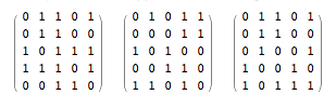
Maybe there’s some other clever trick for recognizing ormats, but I haven’t found it. Let me make the question more concrete. Below are three (0,1) square matrices. Two of them are ormats but the third is not. Can you tell the difference?
If it’s so hard to recognize an ormat, how did I count the ormats among a bunch of randomly generated (o,1) matrices? By hard work: I reconstructed the set of permutations allowed by each matrix. Visualize a permutation as a path threading its way through the matrix from left to right, connecting only non-zero elements and touching each column and each row just once. When you have drawn all possible permutation paths, check to see if every non-zero element is included in at least one path; if so, then the matrix is an ormat. Note that this is not an efficient recognition procedure. In the worst case (namely, an all-ones matrix), there are k! permutations, so this method has exponential running time. But k! is better than \(2^{k^2}\); and, besides, for sparse matrices the number of permutations is much smaller than k!. The 10 × 10 matrix presented as an example at the start of this post gives rise to 580 permutations, a manageable number. Here’s what they look like, plotted as a spider web of red paths across the bar chart.
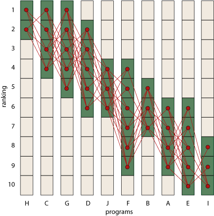
Every nonzero site is visited by at least one permutation path, so this set of rank-intervals is indeed valid.
This process of lacing permutations through a matrix finally brings me back to Question 1, about how to make sense of the NRC’s fuzzy ranking scheme. Let’s take a small example:

Examining the graph above shows that A must rank either first or second—but which is more likely? In the absence of more-detailed information, it seems reasonable to assume the two cases are equally likely; we assign them each a probability of 1/2. Similarly, B has the rank-interval {1–3}, and so we might suppose that each of these three cases has probability 1/3. Continuing in the same way, we assign probabilities to every element of the matrix.
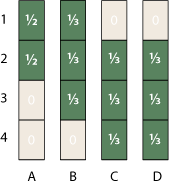
But wait! This can’t be right; our probabilities have sprung a leak. Any proper set of probabilities has to sum to 1. Our procedure assures that each column obeys this rule, but there is no such guarantee for the rows. In row 1, we’re missing one-sixth of our probability, and in row 2 we have an excess of 1/2; row 4 comes up short by 1/3.
Is there any self-consistent assignment of probabilities for the elements of this matrix? Sure. As a matter of fact, there are infinitely many such assignments, including this one:
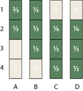
I’ll return in a moment to the question of how I plucked those particular numbers out of the air, but note first what they imply about the ranking of items A through D. For item A, with the rank-interval {1–2}, the odds are two-to-one that it ranks first rather than second. B has the behavior we expected from the outset, with probability uniformly distributed over the three cases. But if you pick either C or D, each with the rank-interval {2–4}, your chance of getting second place is only 1/6, and half the time you’ll be in last place.
Where do these numbers come from? Instead of starting with the assumption that probability is uniformly distributed over each rank-interval, assume that each possible permutation of the ranks is equiprobable. For this matrix there are six allowed permutations: (1, 2, 3, 4), (1, 2, 4, 3), (1, 3, 2, 4), (1, 3, 4, 2), (2, 1, 3, 4) and (2, 1, 4, 3). Observe that four of the six ordering put A first, and only two permutations place A second. We can also tally up such “occupation numbers” for all the other matrix elements:

Dividing these numbers by the total number of permutations, 6, yields the probabilities given above.
We can do the same computation for the 10 × 10 example matrix, which turns out to allow 580 permutations:
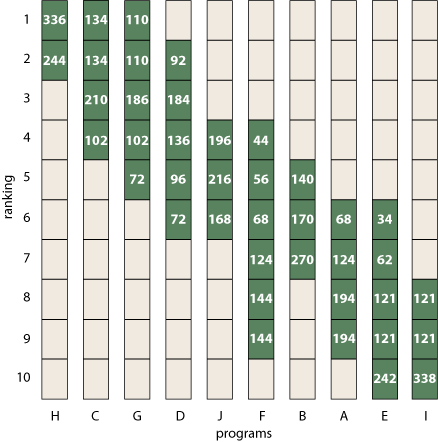
If you care to check, you’ll find that each column and each row sums to 580; dividing all the entries by this number yields a probability matrix with columns and rows that sum to 1 (also known as a doubly stochastic matrix).
This process of tabulating permutation paths recovers some of the information we would have gotten from the arithmetic sum of the permutation matrices—information that was lost in the OR-ing operation. But we get back only some of the information because we have to assume that each permutation included in the OR-sum appears only once. (This is just another way of saying that the allowed permutations are equiprobable.) There’s no particularly good reason to make this assumption, but at least it leads to a feasible probability matrix.
Is there any way of calculating the entries in the doubly stochastic matrix without explicitly tracing out all the permutation paths? I’m sure there is. I think the construction of the matrix can be approached as an integer-programming problem, and perhaps through other kinds of optimization technology. What seems less likely is that there’s some simple and efficient shortcut algorithm. But I could be wrong about that; there’s a lot of mathematics connected with this subject that I don’t understand well enough to write about (e.g., the Birkhoff polytope). I hope others will fill in the gaps.
Getting back to the assessment of grad schools—have we finally found the right way to understand those rank-intervals that the NRC promises to publish any day now? My sense is that a semi-magic square (or, equivalently, a doubly stochastic matrix) will give a less-misleading impression than a simple eyeball sorting on the spans or midpoints of the rank-intervals. But what a lot of bother to get to that point! How many prospective grad students are going to repeat this analysis?
Acknowledgment: Thanks to Geoff Davis of PhDs.org for introducing me to this story. PhDs.org will have the new ratings as soon as the NRC releases them, and may even find a way to make them intelligible! Disclaimer: I’ve done paid work for the PhDs.org web site (but this is not a paid endorsement).
Update 2010-07-27: If you’ve gotten this far, please read the comments as well. A number of commenters have provided important insights and context, which have helped me understand what’s going on in the matrices I’ve been calling ormats. But I’m still a bit murky about the best way to recognize and count them. I’m not sure that publishing my still-murky thoughts is terribly helpful, but maybe someone else will read what follows and give us a dazzling, gemlike synthesis.
For the ormat-recognition problem (Question 4 above), three basic approaches have been mentioned: enumerating the permutation paths through the matrix, examining matrix minors, and looking for perfect matchings in a bipartite graph defined by the matrix. It seems to me that all of these methods are doing the same thing.
Start with Barry Cipra’s method of minors. The basic operation is to choose a nonzero matrix element, then delete the row and the column in which that element occurs. You then apply the same operation to the remaining, smaller matrix.
In tracing permutation paths, we’re looking for sequences of nonzero elements, drawing one element from each column and each row. A way of organizing this search is to choose a nonzero element and then, after recording its location, delete the corresponding column and row, so that no other elements can be chosen from that column or row.
In the method based on Hall’s theorem, as explained by John R., we view the ormat as the adjacency matrix of a bipartite graph, where every nonzero element designates an edge connecting a row vertex to a column vertex. To find a matching, we delete an edge, along with the two vertices it connects (and also all the other edges incident on those vertices). Then we recurse on the smaller remaining graph. (See further update below.) If you translate this operation on the graph back into the language of matrices, deleting an edge and its endpoints amounts to deleting a row and a column of the adjacency matrix.
I am not asserting that these three algorithms are all identical, but they all rely on the same underlying operation. To say more, we would need to consider the control structure of the algorithms—how the basic operations are organized, how the recursion works, all the details of the bookkeeping. I don’t trust myself to make those comparisons without trying to implement the three methods, which I have not yet done. However, at this point I just don’t see how any method can guarantee correct results without something resembling backtracking (or else exhaustive search through an exponential space). After all, we’re not looking for just one matching in the graph, or one decomposition into matrix minors, or one permutation path; we have to examine them all.
Here’s a further hand-wavy argument for the essential difficulty of the task. For a (0,1) matrix, the number of permutation paths that avoid all zero entries is equal to the permanent of the matrix. Computing the permanent of such a matrix is known to be #P-complete.
Update 2010-07-31: With lots of help from my friends, I think I finally get it. Although there could be as many as k! permutation paths in a k × k matrix, you don’t need to examine all of the paths to decide whether or not the matrix is an ormat. It’s enough to establish that one such path passes through each nonzero element. This is what the algorithm based on Hall’s theorem does. As Frans points out in a comment below, I misunderstood the essential nature of that algorithm (in spite of having it explained to me several times). There is no recursive deconstruction into progressively smaller matrix minors; instead, we just loop over all the nonzero elements of the matrix, find the minor associated with each such element, then check for a perfect matching in the minor. (Still more refinements are possible—but already we have a polynomial algorithm.)
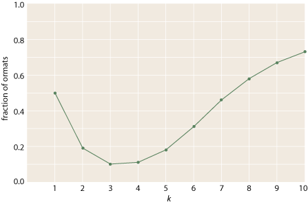
With this efficient recognizer predicate, it’s easy to measure the proportion of ormats in random matrices at larger values of k:
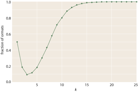
As expected, the fraction of ormats approaches 1 beyond about k = 20.
So much for identifying ormats. I am still unable to extend the series of exact counts beyond k = 5. The tabulations for random (0,1) matrices suggest that for k = 6 there should be about 20 billion ormats, and counting that high is just too painful. I need to work out the symmetries of the problem.
As far as I can tell, assigning exact probabilities to the nonzero matrix elements requires a full enumeration of all the permutation paths, and thus a calculation equivalent to the permanent. There may be a useful approximation.
Barry Cipra asks a really good question: The permanent tells us the maximum number of permutations that could possibly be included in a given ormat, but what is the minimum number? A naive upper bound is the number of 1s in the matrix, but I don’t see an easy path to an exact count. But enough for now.