Getting to Know Julia
by Brian Hayes
Published 22 July 2016
When I first started playing with computers, back in the Pleistocene, writing a few lines of code and watching the machine carry out my instructions was enough to give me a little thrill. “Look! It can count to 10!” Today, learning a new programming language is my way of reviving that sense of wonder.
Lately I’ve been learning Julia, which describes itself as “a high-level, high-performance dynamic programming language for technical computing.” I’ve been dabbling with Julia for a couple of years, but this spring I completed my first serious project—my first attempt to do something useful with the language. I wrote a bunch of code to explore correlations between consecutive prime numbers mod m, inspired by the recent paper of Lemke Oliver and Soundararajan. The code from that project, wrapped up in a Jupyter notebook, is available on GitHub. A bit-player article published last month presented the results of the computation. Here I want to say a few words about my experience with the language.
I also discussed Julia a year ago, on the occasion of JuliaCon 2015, the annual gathering of the Julia community. Parts of this post were written at JuliaCon 2016, held at MIT June 21–25.
This document is itself derived from a Jupyter notebook, although it has been converted to static HTML—meaning that you can only read it, not run the code examples. (I’ve also done some reformatting to save space and improve appearance.) If you have a working installation of Julia and Jupyter, I suggest you download the fully interactive notebook from GitHub, so that you can edit and run the code. If you haven’t installed Julia, download the notebook anyway. You can upload it to JuliaBox.org and run it online. JuliaBox folded up in 2020. See this Discourse thread for some possible alternatives.
What Is Julia?
A 2014 paper by the founders of the Julia project sets an ambitious goal. To paraphrase: There are languages that make programming quick and easy, and there are languages that make computation fast and efficient. The two sets of languages have long been disjoint. Julia aims to fix that. It offers high-level programming, where algorithms are expressed succinctly and without much fussing over data types and memory allocation. But it also strives to match the performance of lower-level languages such as Fortran and C. Achieving these dual goals requires attention both to the design of the language itself and to the implementation.
The Julia project was initiated by a small group at MIT, including Jeff Bezanson, Alan Edelman, Stefan Karpinski, and Viral B. Shah, and has since attracted about 500 contributors. The software is open source, hosted at GitHub.
Who Am I?
In my kind of programming, the end product is not the program itself but the answers it computes. As a result, I favor an incremental and interactive style. I want to write and run small chunks of code—typically individual procedures—without having to build a lot of scaffolding to support them. For a long time I worked mainly in Lisp, although in recent years I’ve also written a fair amount of Python and JavaScript. I mention all this because my background inevitably colors my judgment of programming languages and environments. If you’re a software engineer on a large team building large systems, your needs and priorities are surely different from mine.
What Julia Code Looks Like
Enough generalities. Here’s a bit of Julia code, plucked from my recent project:
# return the next prime after x

# define the function...
function next_prime(x)
    x += iseven(x) ? 1 : 2
    while !isprime(x)
        x += 2
    end
    return x
end

# and now invoke it
next_prime(10000000) ⇒ 10000019
Given an integer x, we add 1 if x is even and otherwise add 2, thereby ensuring that the new value of x is odd. Now we repeatedly check the isprime(x) predicate, or rather its negation !isprime(x). As long as x is not a prime number, we continue incrementing by 2; when x finally lands on a prime value (it must do so eventually, according to Euclid), the while loop terminates and the function returns the prime value of x.
In this code snippet, note the absence of punctuation: No semicolons separate the statements, and no curly braces delimit the function body. The syntax owes a lot to MATLAB—most conspicuously the use of the end keyword to mark the end of a block, without any corresponding begin. The resemblance to MATLAB is more than coincidence; some of the key people in the Julia project have a background in numerical analysis and linear algebra, where MATLAB has long been a standard tool. One of those people is Alan Edelman. I remember asking him, 15 years ago, “How do you compute the eigenvalues of a matrix?” He explained: “You start up MATLAB and type eig.” The same incantation works in Julia.
The sparse punctuation and the style of indentation also make Julia code look a little like Python, but in this case the similarity is only superficial. In Python, indentation determines the scope of statements, but in Julia indentation is merely an aid to the human reader; the program would compute the same result even if all the lines were flush left.
More Basics
The next_prime function above shows a while loop. Here’s a for loop:
# for-loop factorial

function factorial_for(n)
    fact = 1
    for i in 1:n         # i takes each value in 1, 2, ..., n
        fact *= i        # equivalent to fact = fact * i
    end
    return fact
end

factorial_for(10) ⇒ 3628800
The same idea can be expressed more succinctly and idiomatically:
# factorial via range product

function factorial_range(n)
    return prod(1:n)
end

factorial_range(11) ⇒ 39916800
Here 1:n denotes the numeric range \(1, 2, 3, …, n\), and the prod function returns the product of all the numbers in the range. Still too verbose? Using an abbreviated style of function definition, it becomes a true one-liner:
fact_range(n) = prod(1:n)

fact_range(12) ⇒ 479001600
Recursion
As an immigrant from the land of Lisp, I can’t in good conscience discuss the factorial function without also presenting a recursive version:
# recursive definition of factorial

function factorial_rec(n)
    if n < 2
        return 1
    else
        return n * factorial_rec(n - 1)
    end
end

factorial_rec(13) ⇒ 6227020800
You can save some keystrokes by replacing the if... else... end statement with a ternary operator. The syntax is
predicate ? consequent : alternative.
If predicate evaluates to true, the expression returns the value of consequent; otherwise it returns the value of alternative. With this device, the recursive factorial function looks like this:
# recursive factorial with ternary operator

function factorial_rec_ternary(n)
    n < 2 ? 1 : n * factorial_rec_ternary(n - 1)
end

factorial_rec_ternary(14) ⇒ 87178291200
One sour note on the subject of recursion: The Julia compiler does not perform tail-call conversion, which endows recursive procedure definitions with the same space and time efficiency as iterative structures such as while loops. Consider this pair of daisy-plucking procedures:
function she_loves_me(petals)
    petals == 0 ? true : she_loves_me_not(petals - 1)
end

function she_loves_me_not(petals)
    petals == 0 ? false : she_loves_me(petals - 1)
end

she_loves_me(1001) ⇒ false
These are mutually recursive definitions: Control passes back and forth between them until one or the other terminates when the petals are exhausted. The function works correctly on small values of petals. But let’s try a more challenging exercise:
she_loves_me(1000000)

LoadError: StackOverflowError:
while loading In[8], in expression starting on line 1

 in she_loves_me at In[7]:2 (repeats 80000 times)
The stack overflows because Julia is pushing a procedure-call record onto the stack for every invocation of either she_loves_me or she_loves_me_not. These records will never be needed; when the answer (true or false) is finally determined, it can be returned directly to the top level, without having to percolate up through the cascade of stack frames. The technique for eliminating such unneeded stack frames has been well known for more than 30 years. Implementing tail-call optimization has been discussed by the Julia developers but is “not a priority.” For me this is not a catastrophic defect, but it’s a disappointment. It rules out a certain style of reasoning that in some cases is the most direct way of expressing mathematical ideas.
Array Comprehensions
Given Julia’s heritage in linear algebra, it’s no surprise that there are rich facilities for describing matrices and other array-like objects. One handy tool is the array comprehension, which is written as a pair of square brackets surrounding a description of what the compiler should compute to build the array.
A = [x^2 for x in 1:5] ⇒ [1, 4, 9, 16, 25]
The idea of comprehensions comes from the set-builder notation of mathematics. It was adopted in the programming language SETL in the 1960s, and it has since wormed its way into several other languages, including Haskell and Python. But Julia’s comprehensions are unusual: Whereas Python comprehensions are limited to one-dimensional vectors or lists, Julia comprehensions can specify multidimensional arrays.
B = [x^y for x in 1:3, y in 1:3] ⇒

3x3 Array{Int64,2}:
 1  1   1
 2  4   8
 3  9  27
Multidimensionality comes at a price. A Python comprehension can have a filter clause that selects some of the array elements and excludes others. If Julia had such comprehension filters, you could generate an array of prime numbers with an expression like this: [x for x in 1:100 if isprime(x)]. But adding filters to multidimensional arrays is problematic; you can’t just pluck values out of a matrix and keep the rest of the structure intact. Nevertheless, it appears a solution is in hand. After three years of discussion, a fix has recently been added to the code base. (I have not yet tried it out.)
Multiple Dispatch
This sounds like something the 911 operator might do in response to a five-alarm fire, but in fact multiple dispatch is a distinctive core idea in Julia. Understanding what it is and why you might care about it requires a bit of context.
In almost all programming languages, an expression along the lines of x * y multiplies x by y, whether x and y are integers, floating-point numbers, or maybe even complex numbers or matrices. All of these operations qualify as multiplication, but the underlying algorithms—the ways the bits are twiddled to compute the product—are quite different. Thus the * operator is polymorphic: It’s a single symbol that evokes many different actions. One way to handle this situation is to write a single big function—call it mul(x, y)—that has a chain of if... then... else statements to select the right multiplication algorithm for each x, y pair. If you want to multiply all possible combinations of \(n\) kinds of numbers, the if statement needs \(n^2\) branches. Maintaining that monolithic mul procedure can become a headache. Suppose you want to add a new type of number, such as quaternions. You would have to patch in new routines throughout the existing mul code.
When object-oriented programming (OOP) swept through the world of computing in the 1980s, it offered an alternative. In an object-oriented setting, each class of numbers has its own set of multiplication procedures, or methods. Instead of one universal mul function, there’s a mul method for integers, another mul for floats, and so on. To multiply x by y, you don’t write mul(x, y) but rather something like x.mul(y). The object-oriented programmer thinks of this protocol as sending a message to the x object, asking it to apply its mul method to the y argument. You can also describe the scheme as a single-dispatch mechanism. The dispatcher is a behind-the-scenes component that keeps track of all methods with the same name, such as mul, and chooses which of those methods to invoke based on the data type of the single argument x. (The x object still needs some internal mechanism to examine the type of y to know which of its own methods to apply.)
Multiple dispatch is a generalization of single dispatch. The dispatcher looks at all the arguments and their types, and chooses the method accordingly. Once that decision is made, no further choices are needed. There might be separate mul methods for combining two integers, for an integer and a float, for a float and a complex, etc. Julia has 138 methods linked to the multiplication operator *, including a few mildly surprising combinations. (Quick, what’s the value of false * 42?)
# Typing "methods(f)" for any function f, or for an operator
# such as "*", produces a list of all the methods and their
# type signatures. The links take you to the source code.

methods(*) ⇒
- *(x::Bool, y::Bool) at bool.jl:38
- *{T<:Unsigned}(x::Bool, y::T<:Unsigned) at bool.jl:53
- *(x::Bool, z::Complex{Bool}) at complex.jl:122
- *(x::Bool, z::Complex{T<:Real}) at complex.jl:129
- *{T<:Number}(x::Bool, y::T<:Number) at bool.jl:49
- *(x::Float32, y::Float32) at float.jl:211
- *(x::Float64, y::Float64) at float.jl:212
- *(z::Complex{T<:Real}, w::Complex{T<:Real}) at complex.jl:113
- *(z::Complex{Bool}, x::Bool) at complex.jl:123
- *(z::Complex{T<:Real}, x::Bool) at complex.jl:130
- *(x::Real, z::Complex{Bool}) at complex.jl:140
- *(z::Complex{Bool}, x::Real) at complex.jl:141
- *(x::Real, z::Complex{T<:Real}) at complex.jl:152
- *(z::Complex{T<:Real}, x::Real) at complex.jl:153
- *(x::Rational{T<:Integer}, y::Rational{T<:Integer}) at rational.jl:186
- *(a::Float16, b::Float16) at float16.jl:136
- *{N}(a::Integer, index::CartesianIndex{N}) at multidimensional.jl:50
- *(x::BigInt, y::BigInt) at gmp.jl:256
- *(a::BigInt, b::BigInt, c::BigInt) at gmp.jl:279
- *(a::BigInt, b::BigInt, c::BigInt, d::BigInt) at gmp.jl:285
- *(a::BigInt, b::BigInt, c::BigInt, d::BigInt, e::BigInt) at gmp.jl:292
- *(x::BigInt, c::Union{UInt16,UInt32,UInt64,UInt8}) at gmp.jl:326
- *(c::Union{UInt16,UInt32,UInt64,UInt8}, x::BigInt) at gmp.jl:330
- *(x::BigInt, c::Union{Int16,Int32,Int64,Int8}) at gmp.jl:332
- *(c::Union{Int16,Int32,Int64,Int8}, x::BigInt) at gmp.jl:336
- *(x::BigFloat, y::BigFloat) at mpfr.jl:208
- *(x::BigFloat, c::Union{UInt16,UInt32,UInt64,UInt8}) at mpfr.jl:215
- *(c::Union{UInt16,UInt32,UInt64,UInt8}, x::BigFloat) at mpfr.jl:219
- *(x::BigFloat, c::Union{Int16,Int32,Int64,Int8}) at mpfr.jl:223
- *(c::Union{Int16,Int32,Int64,Int8}, x::BigFloat) at mpfr.jl:227
- *(x::BigFloat, c::Union{Float16,Float32,Float64}) at mpfr.jl:231
- *(c::Union{Float16,Float32,Float64}, x::BigFloat) at mpfr.jl:235
- *(x::BigFloat, c::BigInt) at mpfr.jl:239
- *(c::BigInt, x::BigFloat) at mpfr.jl:243
- *(a::BigFloat, b::BigFloat, c::BigFloat) at mpfr.jl:379
- *(a::BigFloat, b::BigFloat, c::BigFloat, d::BigFloat) at mpfr.jl:385
- *(a::BigFloat, b::BigFloat, c::BigFloat, d::BigFloat, e::BigFloat) at mpfr.jl:392
- *{T<:Number}(x::T<:Number, D::Diagonal{T}) at linalg/diagonal.jl:89
- *(x::Irrational{sym}, y::Irrational{sym}) at irrationals.jl:72
- *(y::Real, x::Base.Dates.Period) at dates/periods.jl:55
- *(x::Number) at operators.jl:74
- *(y::Number, x::Bool) at bool.jl:55
- *(x::Int8, y::Int8) at int.jl:19
- *(x::UInt8, y::UInt8) at int.jl:19
- *(x::Int16, y::Int16) at int.jl:19
- *(x::UInt16, y::UInt16) at int.jl:19
- *(x::Int32, y::Int32) at int.jl:19
- *(x::UInt32, y::UInt32) at int.jl:19
- *(x::Int64, y::Int64) at int.jl:19
- *(x::UInt64, y::UInt64) at int.jl:19
- *(x::Int128, y::Int128) at int.jl:456
- *(x::UInt128, y::UInt128) at int.jl:457
- *{T<:Number}(x::T<:Number, y::T<:Number) at promotion.jl:212
- *(x::Number, y::Number) at promotion.jl:168
- *{T<:Union{Complex{Float32},Complex{Float64},Float32,Float64},S} (A::Union{DenseArray{T<:Union{Complex{Float32}, Complex{Float64},Float32,Float64},2}, SubArray{T<:Union{Complex{Float32}, Complex{Float64}, Float32,Float64},2, A<:DenseArray{T,N}, I<:Tuple{Vararg{Union{Colon,Int64,Range{Int64}}}},LD}}, x::Union{DenseArray{S,1}, SubArray{S,1,A<:DenseArray{T,N}, I<:Tuple{Vararg{Union{Colon,Int64,Range{Int64}}}},LD}}) at linalg/matmul.jl:82
- *(A::SymTridiagonal{T}, B::Number) at linalg/tridiag.jl:86
- *(A::Tridiagonal{T}, B::Number) at linalg/tridiag.jl:406
- *(A::UpperTriangular{T,S<:AbstractArray{T,2}}, x::Number) at linalg/triangular.jl:454
- *(A::Base.LinAlg.UnitUpperTriangular{T,S<:AbstractArray{T,2}}, x::Number) at linalg/triangular.jl:457
- *(A::LowerTriangular{T,S<:AbstractArray{T,2}}, x::Number) at linalg/triangular.jl:454
- *(A::Base.LinAlg.UnitLowerTriangular{T,S<:AbstractArray{T,2}}, x::Number) at linalg/triangular.jl:457
- *(A::Tridiagonal{T}, B::UpperTriangular{T,S<:AbstractArray{T,2}}) at linalg/triangular.jl:969
- *(A::Tridiagonal{T}, B::Base.LinAlg.UnitUpperTriangular{T,S<:AbstractArray{T,2}}) at linalg/triangular.jl:969
- *(A::Tridiagonal{T}, B::LowerTriangular{T,S<:AbstractArray{T,2}}) at linalg/triangular.jl:969
- *(A::Tridiagonal{T}, B::Base.LinAlg.UnitLowerTriangular{T,S<:AbstractArray{T,2}}) at linalg/triangular.jl:969
- *(A::Base.LinAlg.AbstractTriangular{T,S<:AbstractArray{T,2}}, B::Base.LinAlg.AbstractTriangular{T,S<:AbstractArray{T,2}}) at linalg/triangular.jl:975
- *{TA,TB}(A::Base.LinAlg.AbstractTriangular{TA,S<:AbstractArray{T,2}}, B:: Union{DenseArray{TB,1},DenseArray{TB,2}, SubArray{TB,1,A<:DenseArray{T,N}, I<:Tuple{Vararg{Union{Colon,Int64,Range{Int64}}}},LD}, SubArray{TB,2,A<:DenseArray{T,N}, I<:Tuple{Vararg{Union{Colon,Int64,Range{Int64}}}},LD}}) at linalg/triangular.jl:989
- *{TA,TB}(A:: Union{DenseArray{TA,1},DenseArray{TA,2}, SubArray{TA,1,A<:DenseArray{T,N}, I<:Tuple{Vararg{Union{Colon,Int64,Range{Int64}}}},LD}, SubArray{TA,2,A<:DenseArray{T,N}, I<:Tuple{Vararg{Union{Colon,Int64,Range{Int64}}}},LD}}, B::Base.LinAlg.AbstractTriangular{TB,S<:AbstractArray{T,2}}) at linalg/triangular.jl:1016
- *{TA,Tb}(A::Union{Base.LinAlg.QRCompactWYQ{TA,M<:AbstractArray{T,2}}, Base.LinAlg.QRPackedQ{TA,S<:AbstractArray{T,2}}}, b:: Union{DenseArray{Tb,1}, SubArray{Tb,1,A<:DenseArray{T,N}, I<:Tuple{Vararg{Union{Colon,Int64,Range{Int64}}}},LD}}) at linalg/qr.jl:166
- *{TA,TB}(A::Union{Base.LinAlg.QRCompactWYQ{TA,M<:AbstractArray{T,2}}, Base.LinAlg.QRPackedQ{TA,S<:AbstractArray{T,2}}}, B:: Union{DenseArray{TB,2},SubArray{TB,2,A<:DenseArray{T,N}, I<:Tuple{Vararg{Union{Colon,Int64,Range{Int64}}}},LD}}) at linalg/qr.jl:178
- *{TA,TQ,N}(A:: Union{DenseArray{TA,N}, SubArray{TA,N,A<:DenseArray{T,N}, I<:Tuple{Vararg{Union{Colon,Int64,Range{Int64}}}},LD}}, Q::Union{Base.LinAlg.QRCompactWYQ{TQ,M<:AbstractArray{T,2}}, Base.LinAlg.QRPackedQ{TQ,S<:AbstractArray{T,2}}}) at linalg/qr.jl:253
- *(A::Union{Hermitian{T,S},Symmetric{T,S}}, B::Union{Hermitian{T,S},Symmetric{T,S}}) at linalg/symmetric.jl:117
- *(A::Union{DenseArray{T,2}, SubArray{T,2, A<:DenseArray{T,N}, I<:Tuple{Vararg{Union{Colon,Int64,Range{Int64}}}},LD}}, B::Union{Hermitian{T,S},Symmetric{T,S}}) at linalg/symmetric.jl:118
- *{T<:Number}(D::Diagonal{T}, x::T<:Number) at linalg/diagonal.jl:90
- *(Da::Diagonal{T}, Db::Diagonal{T}) at linalg/diagonal.jl:92
- *(D::Diagonal{T}, V::Array{T,1}) at linalg/diagonal.jl:93
- *(A::Array{T,2}, D::Diagonal{T}) at linalg/diagonal.jl:94
- *(D::Diagonal{T}, A::Array{T,2}) at linalg/diagonal.jl:95
- *(A::Bidiagonal{T}, B::Number) at linalg/bidiag.jl:192
- *(A::Union{Base.LinAlg.AbstractTriangular{T,S<:AbstractArray{T,2}}, Bidiagonal{T}, Diagonal{T}, SymTridiagonal{T}, Tridiagonal{T}}, B::Union{Base.LinAlg.AbstractTriangular{T, S<:AbstractArray{T,2}}, Bidiagonal{T},Diagonal{T}, SymTridiagonal{T},Tridiagonal{T}}) at linalg/bidiag.jl:198
- *{T}(A::Bidiagonal{T}, B::AbstractArray{T,1}) at linalg/bidiag.jl:202
- *(B::BitArray{2}, J::UniformScaling{T<:Number}) at linalg/uniformscaling.jl:122
- *{T,S}(s::Base.LinAlg.SVDOperator{T,S}, v::Array{T,1}) at linalg/arnoldi.jl:261
- *(S::SparseMatrixCSC{Tv,Ti<:Integer}, J::UniformScaling{T<:Number}) at sparse/linalg.jl:23
- *{Tv,Ti}(A::SparseMatrixCSC{Tv,Ti}, B::SparseMatrixCSC{Tv,Ti}) at sparse/linalg.jl:108
- *{TvA,TiA,TvB,TiB}(A::SparseMatrixCSC{TvA,TiA}, B::SparseMatrixCSC{TvB,TiB}) at sparse/linalg.jl:29
- *{TX,TvA,TiA}(X:: Union{DenseArray{TX,2}, SubArray{TX,2,A<:DenseArray{T,N}, I<:Tuple{Vararg{Union{Colon,Int64,Range{Int64}}}},LD}}, A::SparseMatrixCSC{TvA,TiA}) at sparse/linalg.jl:94
- *(A::Base.SparseMatrix.CHOLMOD.Sparse {Tv<:Union{Complex{Float64},Float64}}, B:: Base.SparseMatrix.CHOLMOD.Sparse{Tv<:Union{Complex{Float64}, Float64}}) at sparse/cholmod.jl:1157
- *(A::Base.SparseMatrix.CHOLMOD.Sparse {Tv<:Union{Complex{Float64},Float64}}, B:: Base.SparseMatrix.CHOLMOD.Dense {T<:Union{Complex{Float64},Float64}}) at sparse/cholmod.jl:1158
- *(A::Base.SparseMatrix.CHOLMOD.Sparse {Tv<:Union{Complex{Float64},Float64}}, B:: Union{Array{T,1},Array{T,2}}) at sparse/cholmod.jl:1159
- *{Ti}(A::Symmetric{Float64,SparseMatrixCSC{Float64,Ti}}, B::SparseMatrixCSC{Float64,Ti}) at sparse/cholmod.jl:1418
- *{Ti}(A::Hermitian{Complex{Float64}, SparseMatrixCSC{Complex{Float64},Ti}}, B::SparseMatrixCSC{Complex{Float64},Ti}) at sparse/cholmod.jl:1419
- *{T<:Number}(x::AbstractArray{T<:Number,2}) at abstractarraymath.jl:50
- *(B::Number, A::SymTridiagonal{T}) at linalg/tridiag.jl:87
- *(B::Number, A::Tridiagonal{T}) at linalg/tridiag.jl:407
- *(x::Number, A::UpperTriangular{T,S<:AbstractArray{T,2}}) at linalg/triangular.jl:464
- *(x::Number, A::Base.LinAlg.UnitUpperTriangular{T, S<:AbstractArray{T,2}}) at linalg/triangular.jl:467
- *(x::Number, A::LowerTriangular{T,S<:AbstractArray{T,2}}) at linalg/triangular.jl:464
- *(x::Number, A::Base.LinAlg.UnitLowerTriangular{T, S<:AbstractArray{T,2}}) at linalg/triangular.jl:467
- *(B::Number, A::Bidiagonal{T}) at linalg/bidiag.jl:193
- *(A::Number, B::AbstractArray{T,N}) at abstractarraymath.jl:54
- *(A::AbstractArray{T,N}, B::Number) at abstractarraymath.jl:55
- *(s1::AbstractString, ss::AbstractString…) at strings/basic.jl:50
- *(this::Base.Grisu.Float, other::Base.Grisu.Float) at grisu/float.jl:138
- *(index::CartesianIndex{N}, a::Integer) at multidimensional.jl:54
- *{T,S}(A::AbstractArray{T,2}, B::Union{DenseArray{S,2}, SubArray{S,2,A<:DenseArray{T,N}, I<:Tuple{Vararg{Union{Colon,Int64,Range{Int64}}}},LD}}) at linalg/matmul.jl:131
- *{T,S}(A::AbstractArray{T,2}, x::AbstractArray{S,1}) at linalg/matmul.jl:86
- *(A::AbstractArray{T,1}, B::AbstractArray{T,2}) at linalg/matmul.jl:89
- *(J1::UniformScaling{T<:Number}, J2::UniformScaling{T<:Number}) at linalg/uniformscaling.jl:121
- *(J::UniformScaling{T<:Number}, B::BitArray{2}) at linalg/uniformscaling.jl:123
- *(A::AbstractArray{T,2}, J::UniformScaling{T<:Number}) at linalg/uniformscaling.jl:124
- *{Tv,Ti}(J::UniformScaling{T<:Number}, S::SparseMatrixCSC{Tv,Ti}) at sparse/linalg.jl:24
- *(J::UniformScaling{T<:Number}, A::Union{AbstractArray{T,1},AbstractArray{T,2}}) at linalg/uniformscaling.jl:125
- *(x::Number, J::UniformScaling{T<:Number}) at linalg/uniformscaling.jl:127
- *(J::UniformScaling{T<:Number}, x::Number) at linalg/uniformscaling.jl:128
- *{T,S}(R::Base.LinAlg.AbstractRotation{T}, A::Union{AbstractArray{S,1},AbstractArray{S,2}}) at linalg/givens.jl:9
- *{T}(G1::Base.LinAlg.Givens{T}, G2::Base.LinAlg.Givens{T}) at linalg/givens.jl:307
- *(p::Base.DFT.ScaledPlan{T,P,N}, x::AbstractArray{T,N}) at dft.jl:262
- *{T,K,N}(p::Base.DFT.FFTW.cFFTWPlan{T,K,false,N}, x::Union{DenseArray{T,N}, SubArray{T,N,A<:DenseArray{T,N}, I<:Tuple{Vararg{Union{Colon,Int64,Range{Int64}}}},LD}}) at fft/FFTW.jl:621
- *{T,K}(p::Base.DFT.FFTW.cFFTWPlan{T,K,true,N}, x::Union{DenseArray{T,N}, SubArray{T,N,A<:DenseArray{T,N}, I<:Tuple{Vararg{Union{Colon,Int64,Range{Int64}}}},LD}}) at fft/FFTW.jl:628
- *{N}(p::Base.DFT.FFTW.rFFTWPlan{Float32,-1,false,N}, x:: Union{DenseArray{Float32,N}, SubArray{Float32,N,A<:DenseArray{T,N}, I<:Tuple{Vararg{Union{Colon,Int64,Range{Int64}}}},LD}}) at fft/FFTW.jl:698
- *{N}(p::Base.DFT.FFTW.rFFTWPlan{Complex{Float32},1,false,N}, x::Union{DenseArray{Complex{Float32},N}, SubArray{Complex{Float32},N,A<:DenseArray{T,N}, I<:Tuple{Vararg{Union{Colon,Int64,Range{Int64}}}},LD}}) at fft/FFTW.jl:705
- *{N}(p::Base.DFT.FFTW.rFFTWPlan{Float64,-1,false,N}, x:: Union{DenseArray{Float64,N}, SubArray{Float64,N,A<:DenseArray{T,N}, I<:Tuple{Vararg{Union{Colon,Int64,Range{Int64}}}},LD}}) at fft/FFTW.jl:698
- *{N}(p::Base.DFT.FFTW.rFFTWPlan{Complex{Float64},1,false,N}, x:: Union{DenseArray{Complex{Float64},N}, SubArray{Complex{Float64},N,A<:DenseArray{T,N}, I<:Tuple{Vararg{Union{Colon,Int64,Range{Int64}}}},LD}}) at fft/FFTW.jl:705
- *{T,K,N}(p::Base.DFT.FFTW.r2rFFTWPlan{T,K,false,N}, x:: Union{DenseArray{T,N}, SubArray{T,N,A<:DenseArray{T,N}, I<:Tuple{Vararg{Union{Colon,Int64,Range{Int64}}}},LD}}) at fft/FFTW.jl:866
- *{T,K}(p::Base.DFT.FFTW.r2rFFTWPlan{T,K,true,N}, x:: Union{DenseArray{T,N}, SubArray{T,N,A<:DenseArray{T,N}, I<:Tuple{Vararg{Union{Colon,Int64,Range{Int64}}}},LD}}) at fft/FFTW.jl:873
- *{T}(p::Base.DFT.FFTW.DCTPlan{T,5,false}, x:: Union{DenseArray{T,N}, SubArray{T,N,A<:DenseArray{T,N}, I<:Tuple{Vararg{Union{Colon,Int64,Range{Int64}}}},LD}}) at fft/dct.jl:188
- *{T}(p::Base.DFT.FFTW.DCTPlan{T,4,false}, x::Union{DenseArray{T,N}, SubArray{T,N,A<:DenseArray{T,N}, I<:Tuple{Vararg{Union{Colon,Int64,Range{Int64}}}},LD}}) at fft/dct.jl:191
- *{T,K}(p::Base.DFT.FFTW.DCTPlan{T,K,true}, x::Union{DenseArray{T,N}, SubArray{T,N,A<:DenseArray{T,N}, I<:Tuple{Vararg{Union{Colon,Int64,Range{Int64}}}},LD}}) at fft/dct.jl:194
- *{T}(p::Base.DFT.Plan{T}, x::AbstractArray{T,N}) at dft.jl:221
- *(?::Number, p::Base.DFT.Plan{T}) at dft.jl:264
- *(p::Base.DFT.Plan{T}, ?::Number) at dft.jl:265
- *(I::UniformScaling{T<:Number}, p::Base.DFT.ScaledPlan{T,P,N}) at dft.jl:266
- *(p::Base.DFT.ScaledPlan{T,P,N}, I::UniformScaling{T<:Number}) at dft.jl:267
- *(I::UniformScaling{T<:Number}, p::Base.DFT.Plan{T}) at dft.jl:268
- *(p::Base.DFT.Plan{T}, I::UniformScaling{T<:Number}) at dft.jl:269
- *{P<:Base.Dates.Period} (x::P<:Base.Dates.Period, y::Real) at dates/periods.jl:54
- *(a, b, c, xs…) at operators.jl:103
Before Julia came along, the best-known example of multiple dispatch was the Common Lisp Object System, or CLOS. As a Lisp guy, I’m familiar with CLOS, but I’ve seldom found it useful; it’s too heavy a hammer for most of my little nails. But whereas CLOS is an optional add-on to Lisp, multiple dispatch is deeply embedded in the infrastructure of Julia. You can’t really ignore it.
Multiple dispatch encourages a style of programming in which you write an abundance of short, single-purpose methods that handle specific combinations of argument types. This is surely an improvement over writing one huge function with an internal tangle of spaghetti logic to handle dozens special cases. The Julia documentation offers this example:
# roll-your-own method dispatch

function norm(A)
    if isa(A, Vector)
        return sqrt(real(dot(A,A)))
    elseif isa(A, Matrix)
        return max(svd(A)[2])
    else
        error("norm: invalid argument")
    end
end

# let the compiler do method dispatch

norm(x::Vector) = sqrt(real(dot(x,x)))
norm(A::Matrix) = max(svd(A)[2])

# Note: The 'x::y syntax declares that variable x will have
# a value of type y.
Splitting the procedure into two methods makes the definition clearer and more concise, and it also promises better performance. There’s no need to crawl through the if... else... chain at runtime; the appropriate method is chosen at compile time.
That example seems pretty compelling. Edelman gives another illuminating demo, defining tropical arithmetic in a few lines of code. (In tropical arithmetic, plus is min and times is plus.)
Unfortunately, my own attempts to structure code in this way have not been so successful. Take the next_prime(x) function shown at the beginning of this notebook. The argument x might be either an ordinary integer (some subtype of Int, such as Int64) or a BigInt, a numeric type accommodating integers of unbounded size. So I tried writing separate methods next_prime(x::Int) and next_prime(x::BigInt). The result, however, was annoying code duplication: The bodies of those two methods were identical. Furthermore, splitting the two methods yielded no performance gain; the compiler was able to produce efficient code without any type annotations at all.
I remain somewhat befuddled about how best to exploit multiple dispatch. Suppose you are creating a graphics program that can plot either data from an array or a mathematical function. You could define a generic plot procedure with two methods:
function plot(data::Array)
    # ... code for array plotting
end

function plot(fn::Function)
    # ... code for function plotting
end
With these definitions, calls to plot([2, 4, 6, 8]) and plot(sin) would automatically be routed to the appropriate method. However, making the two methods totally independent is not quite right either. They both need to deal with scales, grids, tickmarks, labels, and other graphics accoutrements. I’m still learning how to structure such code. No doubt it will become clearer with experience; in the meantime, advice is welcome.
Multiple dispatch is not a general pattern-matching mechanism. It discriminates only on the basis of the type signature of a function’s arguments, not on the values of those arguments. In Haskell—a language that does have pattern matching—you can write a function definition like this:
factorial 0 = 1
factorial n = n * factorial (n - 1)
That won’t work in Julia. (Actually, there may be a baroque way to do it, but it’s not recommended.) (And I’ve just learned there’s a pattern-matching package.) (And another.)
Multiple dispatch vs. OOP
In CLOS, multiple dispatch is an adjunct to an object-oriented programming system; in Julia, multiple dispatch is an alternative to OOP, and perhaps a repudiation of it. OOP is a noun-centered protocol: Objects are things that own both data and procedures that act on the data. Julia is verb-centered: Procedures (or functions) are the active elements of a program, and they can be applied to any data, not just their own private variables. The Julia documentation notes:
Multiple dispatch is particularly useful for mathematical code, where it makes little sense to artificially deem the operations to “belong” to one argument more than any of the others: does the addition operation in
x + ybelong toxany more than it does toy? The implementation of a mathematical operator generally depends on the types of all of its arguments. Even beyond mathematical operations, however, multiple dispatch ends up being a powerful and convenient paradigm for structuring and organizing programs.
I agree about the peculiar asymmetry of asking x to add y to itself. And yet that’s only one small aspect of what object-oriented programming is all about. There are many occasions when it’s really handy to bundle up related code and data in an object, if only for the sake of tidyness. If I had been writing my primes program in an object-oriented language, I would have created a class of objects to hold various properties of a sequence of consecutive primes, and then instantiated that class for each sequence I generated. Some of the object fields would have been simple data, such as the length of the sequence. Others would have been procedures for calculating more elaborate statistics. Some of the data and procedures would have been private—accessible only from within the object.
No such facility exists in Julia, but there are other ways of addressing some of the same needs. Julia’s user-defined composite types look very much like objects in some respects; they even use the same dot notation for field access that you see in Java, JavaScript and Python. A type definition looks like this.
type Location
    latitude::Float64
    longitude::Float64
end
Given a variable of this type, such as Paris = Location(48.8566, 2.3522), you can access the two fields as Paris.latitude and Paris.longitude. You can even have a field of type Function inside a composite type, as in this declaration:
type Location
    latitude::Float64
    longitude::Float64
    distance_to_pole::Function
end
Then, if you store an appropriate function in that field, you can invoke it as Paris.distance_to_pole(). However, the function has no special access to the other fields of the type; in particular, it doesn’t know which Location it’s being called from, so it doesn’t work like an OOP method.
Julia also has modules, which are essentially private namespaces. Only variables that are explicitly marked as exported can be seen from outside a module. A module can encapsulate both code and data, and so it is probably the closest approach to objects as a mechanism of program organization. But there’s still nothing like the this or self keyword of true object-oriented languages.
Is it brave or foolish, at this point in the history of computer science, to turn your back on the object-oriented paradigm and try something else? It’s surely bold. Two or three generations of programmers have grown up on a steady diet OOP. On the other hand, we have not yet found the One True Path to software wisdom, so there’s surely room for exploring other corners of the ecosystem.
Exactness
A language for “technical computing” had better have strong numerical abilities. Julia has the full gamut of numeric types, with integers of various fixed sizes (from 8 bits to 128 bits), both signed and unsigned, and a comparable spectrum of floating-point precisions. There are also BigInts and BigFloats that expand to accommodate numbers of any size (up to the bounds of available memory). And you can do arithmetic with complex numbers and exact rationals.
This is a well-stocked toolkit, suitable for many kinds of computations. However, the emphasis is on fast floating-point arithmetic with real or complex values, approximated at machine precision. If you want to work in number theory, combinatorics, or cryptography—fields that require exact integers and rational numbers of unbounded size—the tools are provided, but using them requires some extra contortions.
To my taste, the most elegant implementation of numeric types is found in the Scheme programming language, a dialect of Lisp. The Scheme numeric “tower” begins with integers at its base. The integers are a subset of the rational numbers, which in turn are a subset of the reals, which are a subset of the complex numbers. Alongside this hierarchy, and orthogonal to it, Scheme also distinguishes between exact and inexact numbers. Integers and rationals can be represented exactly in a computer system, but many real and complex values can only be approximated, usually by floating-point numbers. In doing basic arithmetic, the Scheme interpreter or compiler preserves exactness. This is easy when you’re adding, subtracting, or multiplying integers, since the result is also invariably an integer. With division of integers, Scheme returns an integer when possible (e.g., \(15 \div 3 = 5\)) and otherwise an exact rational (\(4 \div 6 = 2/3\)). Some Schemes go a step further and return exact results for operations such as square root, when it’s possible to do so (\(\sqrt{4/9} = 2/3\); but \(\sqrt{5} = 2.236068\); the latter is inexact). These are numbers you can count on; they mostly obey well-known principles of mathematics, such as \(\frac{m}{n} \times \frac{n}{m} = 1\).
Julia has the same tower of numeric types, but it is not so scrupulous about exact and inexact values. Consider this series of results:
15 / 3 ⇒ 5.0

4 / 6 ⇒ 0.6666666666666666

(15 / 17) * (17 / 15) ⇒ 0.9999999999999999
Even when the result of dividing two integers is another integer, Julia converts the quotient to a floating-point value (signaled by the presence of a decimal point). We also get floats instead of exact rationals for noninteger quotients. Because exactness is lost, mathematical identities become unreliable.
I think I know why the Julia designers chose this path. It’s all about type stability. The compiler can produce faster code if the output type of a method is always the same. If division of integers could yield either an integer or a float, the result type would not be known until runtime. Using exact rationals rather than floats would impose a double penalty: Rational arithmetic is much slower than (hardware-assisted) floating point.
Given the priorities of the Julia project, consistent floating-point quotients were probably the right choice. I’ll concede that point, but it still leaves me grumpy. I’m tempted to ask, “Why not just make all numbers floating point, the way JavaScript does?” Then all arithmetic operations would be type stable by default. (This is not a serious proposal. I deplore JavaScript’s all-float policy.)
Julia does offer the tools to build your own procedures for exact arithmetic. Here’s one way to conquer divide:
function xdiv(x::Int, y::Int)
    q = x // y                 # yields rational quotient
    den(q) == 1 ? num(q) : q   # return int if possible
end

xdiv(15, 5) ⇒ 3

xdiv(15, 9) ⇒ 5//3
My Int Overfloweth
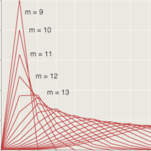
Another numerical quirk gives me the heebie-jeebies. Let’s look again at one of those factorial functions defined above (it doesn’t matter which one).
# run the factorial function f on integers from 1 to limit

function test_factorial(f::Function, limit::Int)
    for n in 1:limit
        @printf("n = %d, f(n) = %d\n", n, f(n))
    end
end

test_factorial(factorial_range, 25) ⇒

n = 1, f(n) = 1
n = 2, f(n) = 2
n = 3, f(n) = 6
n = 4, f(n) = 24
n = 5, f(n) = 120
n = 6, f(n) = 720
n = 7, f(n) = 5040
n = 8, f(n) = 40320
n = 9, f(n) = 362880
n = 10, f(n) = 3628800
n = 11, f(n) = 39916800
n = 12, f(n) = 479001600
n = 13, f(n) = 6227020800
n = 14, f(n) = 87178291200
n = 15, f(n) = 1307674368000
n = 16, f(n) = 20922789888000
n = 17, f(n) = 355687428096000
n = 18, f(n) = 6402373705728000
n = 19, f(n) = 121645100408832000
n = 20, f(n) = 2432902008176640000
n = 21, f(n) = -4249290049419214848
n = 22, f(n) = -1250660718674968576
n = 23, f(n) = 8128291617894825984
n = 24, f(n) = -7835185981329244160
n = 25, f(n) = 7034535277573963776
Everything is copacetic through \(n = 20\), and then suddenly we enter an alternative universe where multiplying a bunch of positive integers gives a negative result. You can probably guess what’s happening here. The computation is being done with 64-bit, twos-complement signed integers, with the most-significant bit representing the sign. When the magnitude of the number exceeds \(2^{63} - 1\), the bit pattern is interpreted as a negative value; then, at \(2^{64}\), it crosses zero and becomes positive again. Essentially, we’re doing arithmetic modulo \(2^{64}\), with an offset.
When a number grows beyond the space allotted for it, something has to give. In some languages the overflowing integer is gracefully converted to a bignum format, so that it can keep growing without constraint. Most Lisps are in this family; so is Python. JavaScript, with its all-floating-point arithmetic, gives approximate answers beyond \(20!\), and beyond \(170!\) all results are deemed equal to Infinity. In several other languages, programs halt with an error message on integer overflow. C is one language that has the same wraparound behavior as Julia. (Actually, the C standard says that signed-integer overflow is “undefined,” which means the compiler can do anything it pleases; but the C compiler I just tested does a wraparound, and I think that’s the common policy.)
The Julia documentation includes a thorough and thoughtful discussion of integer overflow, defending the wraparound strategy by showing that all the alternatives are unacceptable for one reason or another. But even if you go along with that conclusion, you might still feel that wraparound is also unacceptable.
Casual disregard of integer overflow has produced some notably stinky bugs, causing everything from video-game glitches in Pac Man and Donkey Kong to the failure of the first Ariane 5 rocket launch. Dietz, Li, Regehr, and Adve have surveyed bugs of this kind in C programs, finding them even in a module called SafeInt that was specifically designed to protect against such errors. In my little prime-counting project with Julia, I stumbled over overflow problems several times, even after I understood exactly where the risks lay.
In certain other contexts Julia doesn’t play quite so fast and loose. It does runtime bounds checking on array references, throwing an error if you ask for element five of a four-element vector. But it also provides a macro (@inbounds) that allows self-confident daredevils to turn off this safeguard for the sake of speed. Perhaps someday there will be a similar option for integer overflows.
Until then, it’s up to us to write in any overflow checks we think might be prudent. The Julia developers themselves have done so in many places, including their built-in factorial function. See error message below.
test_factorial(factorial, 25) ⇒

n = 1, f(n) = 1
n = 2, f(n) = 2
n = 3, f(n) = 6
n = 4, f(n) = 24
n = 5, f(n) = 120
n = 6, f(n) = 720
n = 7, f(n) = 5040
n = 8, f(n) = 40320
n = 9, f(n) = 362880
n = 10, f(n) = 3628800
n = 11, f(n) = 39916800
n = 12, f(n) = 479001600
n = 13, f(n) = 6227020800
n = 14, f(n) = 87178291200
n = 15, f(n) = 1307674368000
n = 16, f(n) = 20922789888000
n = 17, f(n) = 355687428096000
n = 18, f(n) = 6402373705728000
n = 19, f(n) = 121645100408832000
n = 20, f(n) = 2432902008176640000

LoadError: OverflowError()
while loading In[19], in expression starting on line 1

 in factorial_lookup at combinatorics.jl:29
 in factorial at combinatorics.jl:37
 in test_factorial at In[18]:5
Julia is gaining traction in scientific computing, in finance, and other fields; it has even been adopted as the specification language for an aircraft collision-avoidance system. I do hope that everyone is being careful.
Batteries Installed
“Batteries included” is a slogan of the Python community, boasting that everything you need is provided in the box. And indeed Python comes with a large standard library, supplemented by a huge variety of user-contributed modules (the PyPI index lists about 85,000 of them). On the other hand, although batteries of many kinds are included, they are not installed by default. You can’t accomplish much in Python without first importing a few modules. Just to take a square root, you have to import math. If you want complex numbers, they’re in a different module, and rationals are in a third.
In contrast, Julia is refreshingly self-contained. The standard library has a wide range of functions, and they’re all immediately available, without tracking down and loading external files. There are also about a thousand contributed packages, but you can do quite a lot of useful computing without ever glancing at them. In this respect Julia reminds me of Mathematica, which also tries to put all the commonly needed tools at your fingertips.
A Julia sampler: you get sqrt(x) of course. Also cbrt(x) and hypot(x, y) and log(x) and exp(x). There’s a full deck of trig functions, both circular and hyperbolic, with a variant subset that take their arguments in degrees rather than radians. For combinatorialists we have the factorial function mentioned above, as well as binomial, and various kinds of permutations and combinations. Number theorists can test numbers for primality, and factor those that are composite, calculate gcds and lcms, and so on. Farther afield we have beta, gamma, digamma, eta, and zeta functions, Airy functions, and a dozen kinds of Bessel functions.
For me Julia is like a well-equipped playground, where I can scamper from the swings to the teeter-totter to the monkey bars. At the recent JuliaCon Stefan Karpinsky mentioned a plan to move some of these functions out of the automatically loaded Base module into external libraries. My request: Please don’t overdo it.
Incremental Programming
Julia works splendidly as a platform for incremental, interactive, exploratory programming. There’s no need to write and compile a program as a monolithic structure, with a main function as entry point. You can write a single procedure, immediately compile it and run it, test it, modify it, and examine the assembly code generated by the compiler. It’s ad hack programming at its best.
To support this style of work and play, Julia comes with a built-in REPL, or read-eval-print loop, that operates from a command-line interface. Type an expression at the prompt, press enter, and the system executes the code (compiling if necessary); the value is printed, followed by a new prompt for the next command:

The REPL is pretty good, but I prefer working in a Jupyter notebook, which runs in a web browser. There’s also a development environment called Juno, but I haven’t yet done much with it.
An incremental and iterative style of development can be a challenge for the compiler. When you process an entire program in one piece, the compiler starts from a blank slate. When you compile individual functions, which need to interact with functions compiled earlier, it’s all too easy for the various parts of the system to get out of sync. Gears may fail to mesh.
Problems of this kind can come up with any language, but multiple dispatch introduces some unique quirks. Suppose you’re writing Julia code in a Jupyter notebook. You write and compile a function f(x), which the system accepts as a “generic function with one method.” Later you realize that f should have been a function of two arguments, and so you go back to edit the definition. The modified source code now reads f(x, y). In most languages, this new definition of f would replace the old one, which would thereafter cease to exist. But in Julia you have haven’t replaced anything; instead you now have a “generic function with 2 methods.” The first definition is still present and active in the internal workspace, and so you can call both f(x) and f(x, y). However, the source code for f(x) is nowhere to be found in the notebook. Thus if you end the Jupyter session and later reload the file, any calls to f(x) will produce an error message.
A similar but subtler problem with redefinitions has been a subject of active discussion among the Julia developers for almost five years. There’s hope for a fix in the next major release.
If redefining a function during an interactive session can lead to confusion, trying to redefine a custom type runs into an impassable barrier. Types are immutable. Once defined, they can’t be modified in any way. If you create a type T with two fields a and b, then later decide you also need a field c, you’re stuck. The only way to redefine the type is to shut down the session and restart, losing all computations completed so far. How annoying. There’s a workaround: If you put the type definition inside a module, you can simply reload the module.
Idiosyncrasies
Sometimes it’s the little things that arouse the most heated controversy.
In counting things, Julia generally starts with 1. A vector with n elements is indexed from 1 through n. This is also the default convention in Fortran, MATLAB, Mathematica, and a few other languages; the C family, Python, and JavaScript count from 0 through n-1. The wisdom of 1-based indexing has been a subject of long and spirited debate on the Julia issues forum, on the developer mailing list, and on StackOverflow.
Programs where the choice of indexing origin makes any difference are probably rare, but as it happens my primes study was one of them. I was looking at primes reduced modulo \(m\), and counting the number of primes in each of the \(m\) possible residue classes. Since the residues range from \(0\) to \(m - 1\), it would have been convenient to store the counts in an array with those indices. However, I did not find it terribly onerous to add \(1\) to each index.
Blessedly, the indexing war may soon be over. Tim Holy, a biologist and intrepid Julia contributor, discovered a way to give users free choice of indexing with only a few lines of code and little cost in efficiency. An experimental version of this new mechanism is in the 0.5 developer release.
After the indexing truce, we can still fight over the storage order for arrays and matrices. Julia again follows the precedent of Fortran and MATLAB, reading arrays in column-major order. Given the matrix
$$\begin{matrix}
x_{11} & x_{12} & x_{13} \\
x_{21} & x_{22} & x_{23} \\
\end{matrix}$$
Julia will serialize the elements as \(x_{11}, x_{21}, x_{12}, x_{22}, x_{13}, x_{23}\). C and many other recent languages read across the rows rather than down the columns. This is another largely arbitrary convention, although it may be of some practical importance that most graphic formats are row-major.
Finally there’s the pressing question of what symbol to choose for the string-concatenation operator. Where Python has "abc" + "def" ⇒ "abcdef", Julia does "abc" * "def" ⇒ "abcdef". The reason cited is pretty doctrinaire: In abstract algebras, ‘+’ generally denotes a commutative operation, and string concatenation is not commutative. If you’d like to know more, see the extensive, long-running discussion.
Documentation
The official online documentation is reasonably complete, consistent, and clearly written, but it gives too few examples. Moreover, the organization is sometimes hard to fathom. For example, there’s a chapter on “Multidimensional Arrays” and another titled “Arrays”; I’m often unsure where to look first.
Some of the contributed packages have quite sparse documentation. I made heavy use of a graphics package called GadFly, which is a Julia version of the R package called ggplot2. I had a hard time getting started with the supplied documentation, until I realized that GadFly is close enough to ggplot2 that I could rely on the manual for the latter program.
The simple advice when you’re stumped is: Read the source, Luke. It’s all readily available and easily searched. And almost everything is written in Julia, so you’ll not only find the answers to your questions but also see instructive examples of idiomatic usage.
A few other online resources:
-
Julia by Example (Samuel Colvin)
-
Learn X in Y Minutes, Where X = Julia (Leah Hanson and others)
-
Introducing Julia (a Wikibook)
-
The Julia Express (Bogumił Kamínski)
-
Videos of the talks from JuliaCon 2016 are on YouTube.
As far as I know, Julia has no standard or specification document, which is an interesting absence. For a long time, programming languages had rather careful, formal descriptions of syntax and semantics, laying out exactly which expressions were legal and meaningful in a program. Sometimes the standard came first, before anyone tried to write a compiler or interpreter; Algol 60 was the premier example of this discipline. Sometimes the standard came after, as a device to reconcile diverging implementations; this was the situation with Lisp and C. For now, at least, Julia is apparently defined only by its evolving implementation. Where’s the BNF?
The Future
The rise and fall of programming languages seems to be governed by a highly nonlinear dynamic. Why is Python so popular? Because it’s so popular! With millions of users, there are more add-on packages, more books and articles, more conferences, more showcase applications, more jobs for Python programmers, more classes where Python is the language of instruction. Success breeds success. It’s a bandwagon effect.
If this rich-get-richer economy were the whole story, the world would have only one viable programming language. But there’s a price to be paid for popularity: The overcrowded bandwagon gets trapped in its own wheel ruts and becomes impossible to steer. Think of those 85,000 Python packages. If an improvement in the core language is incompatible with too much of that existing code, the change can be made only with great effort. For example, persuading Python users to migrate from version 2 to version 3 has taken eight years, and the transition is not complete yet.
Julia is approaching the moment when these contrary imperatives—to gain momentum but to stay maneuverable—both become powerful. At the recent JuliaCon, Stefan Karpinsky gave a talk on the path to version 1.0 and beyond. The audience listened with the kind of studious attention that Janet Yellin gets when she announces Fed policy on inflation and interest rates. Toward the end, Karpinsky unveiled the plan: to release version 1.0 within a year, by the time of the 2017 JuliaCon. Cheers and applause.
The 1.0 label connotes maturity—or at least adulthood. It’s a signal that the language is out of school and ready for work in the real-world. And thus begins the struggle to gain momentum while continuing to innovate. For members of Julia’s developer group, there might be a parallel conflict between making a living and continuing to have fun. I’m fervently hoping all these tensions can be resolved.
Will Julia attract enough interest to grow and thrive? I feel I can best address that question by turning it back on myself. Will I continue to write code in Julia?
I’ve said that I do exploratory programming, but I also do expository programming. Computational experiments are an essential part of my work as a science writer. They help me understand what I’m writing about, and they also aid in the storytelling process, through simulations, computer-generated illustrations, and interactive gadgets. Although only a small subset of my readers ever glance at the code I publish, I want to maximize their number and do all I can to deepen their engagement—enticing them to read the code, run it, modify it, and ideally build on it. At this moment, Julia is not the most obvious choice for reaching a broad audience of computational dabblers, but I think it has considerable promise. In some respects, getting started with Julia is easier than it is with Python, if only because there’s less prior art—less to install and configure. I expect to continue working in other languages as well, but I do want to try some more Julia experiments.
Responses from readers:
Please note: The bit-player website is no longer equipped to accept and publish comments from readers, but the author is still eager to hear from you. Send comments, criticism, compliments, or corrections to brian@bit-player.org.
Publication history
First publication: 22 July 2016
Converted to Eleventy framework: 22 April 2025
Update on JuliaBox: 16 May 2025

next_prime(1) fails.
Thanks for the very readable intro to Julia.
Yes,
next_prime(1)fails. In the context of my program it can’t happen, but it’s an ugly wart all the same, especially given how I was going on about mathematical purity and all.Is it even worthwhile to sieve out even numbers? One could just leave that to
isprime(n), where the very first operation of the method forn::Integeris:(n < 3 || iseven(n)) && return n == 2.But I’m mostly concerned about performance with
n::BigInt. Here the issue is not avoiding a primality check for an even number; it’s avoiding constructing the number at all. Supposenis a 2,000-bit number. For each successive value ofn, we’ve got to allocate a block of memory and build the representation of the number; that’s expensive enough to be worth the trouble of sieving out small divisors, I think.Here’s a more general question. The underlying GMP engine that does bignum arithmetic for Julia is capable of doing an update in place. That is, when you evaluate
n += 2, GMP can reuse the existing location ofnrather than allocate new memory. But, if I understand correctly, Julia does not exploit this shortcut because all numbers, including BigInts, are considered immutable. Is there a workaround?Finally, I believe that the right way to fix
next_prime(n)is to get rid of it altogether and use the built-in functionprimes(lo, hi). I didn’t do that because I didn’t want all primes betweenloandhibut rather the nextkprimes afterlo. But most likely it would have been simpler and perhaps faster to useprimes(lo, hi)and afterwards trim or extend the list as needed.You can just do `next_prime(x::Integer)` and that would allow and specialize on any kind of integer (Int32, BigInt, etc.)
With Julia meta programming you can still do a lot of stuff yourself instead of waiting for the language developers to implement and merge into Julia itself, as a Lisper you must love this I think? :)
Here is a @vcomp (vector comprehension) macro that let’s you filter a la Python, with this syntax:
julia> @vcomp Int[i^2 for i in 1:10] when i % 2 == 0
5-element Array{Int,1}:
4
16
36
64
100
* @vcomp macro
It may not be the best implementation, but it works for me.
Thanks for that. I didn’t get around to mentioning metaprogramming, so I’m glad you brought it up.
I think your plot() example can be generalized slightly to provide an instance where multiple dispatch is truly useful.
In my work, we often want to output data in different modalities. For example, I might want to plot a sparse matrix, or save it in an HDF5 file. Thus there are many kinds of output objects and also many kinds of matrix formats (or other data structures) that you want to output. Multiple dispatch provides a clean way to organize the largely independent code in all these choices.
“I remain somewhat befuddled about how best to exploit multiple dispatch”. Then you remain befuddled about why Julia is fast! Multiple dispatch isn’t just part of Julia, multiple dispatch is the core of Julia which allows it to get the performance that it.
Julia uses a JIT to compile code. That’s fine, but you still won’t get major performance improvements if you don’t have type-stability because the compiled code would have to have a lot of cruft to deal with changing representations. However, with multiple dispatch you can easily write a function which compiles into many different methods, and multiple dispatch will choose the appropriate compiled method.
For example, you can make a foo(::Float64) command which works on floats. The compiler can then do a bunch of float specific optimizations. Then you can have a foo(::Int64) method. It can be a completely different underlying algorithm, or it might just convert the int to a float and call foo(::Float64). However, if you were to just make a foo(::Number), then the compiled code would have to be able to handle floats and ints, and have to do a bunch of type-checking at each method call, etc. However, by using multiple dispatch with foo(::Float64) and foo(::Int64), we can call foo(x) when x is a number without thinking about it, but in each case it’s actually calling a compiler-optimized function (and sometimes type-specific optimized algorithm).
So multiple dispatch with together with type-stable functions makes every thing “look like a scripting language”, but in actuality all of the actual code compiles down to pretty much optimal C functions. That is why Julia works so well, and that is the design choice that allows it to excel in performance over the other languages.
That’s not quite right, is it? You can make a foo(::Number) method and still have the compiler automatically generate specialized code for each concrete input type. You do not generally have to make a separate (and identical) implementation for each type, which seems to be exactly the misunderstanding the OP is labouring under.
I’m the befuddled OP, though growing a little less befuddled with the help provided here. Thanks.
I was just trying to make it as explicit as possible [my example in mind was implementing +, which has to call different machine instructions]. But yes, if you make a function where all of the functions it calls inside are defined on the abstract type Number, then foo(::Number) works by essentially making a foo(::T) for each subtype of number that you give it (compiling the first type you give it a new type, or using a precompiled version if in a package). And this is the feature that then makes Julia build up like it is a scripting language. But while having this foo(::Number) as a very different in implementation than what you’d get from other scripting languages.
But there is still an issue if if you make a foo(::Number) and then do a type-conversion of all of the numbers to a concrete type. It still works by multiple dispatch, but if at the top you type check and convert things to either Floats or Rationals depending on whether what comes in is an Integer or Float, then you’ll have a type instability. Instead you should make your function call a function which works on foo(::Number) without having to do any conversions and it will optimize via multiple dispatch. See “Separate kernel functions” in http://docs.julialang.org/en/release-0.4/manual/performance-tips/ .
So I should’ve added a detail: at the bottom each dispatch had to be defined, but when you build up, you have +(::Number,::Number) and the like already defined on each number, so if you just call +, the compiler will be able to choose the right + function and make it efficient (if your types are stable).
Here are a couple of your examples in Haskell.
factorial n = product [1 .. n]
she_loves_me petals
| petals == 0 = True
| otherwise = she_loves_me_not (petals - 1);
she_loves_me_not petals
| petals == 0 = False
| otherwise = she_loves_me (petals - 1)
Neither had any problem executing
> factorial 21
51090942171709440000
> she_loves_me 1000000
True
(Sorry. I didn’t realize I would have to put in the extra new lines and spaces explicitly.)
Here are a couple of your examples in Haskell.
factorial n = product [1 .. n]
she_loves_me petals
| petals == 0 = True
| otherwise = she_loves_me_not (petals - 1)
she_loves_me_not petals
| petals == 0 = False
| otherwise = she_loves_me (petals - 1)
Neither had any problem executing
> factorial 21
51090942171709440000
> she_loves_me 1000000
True
Sorry to put you through such formatting torture.
Haskell is a special case. As a “lazy” language, it doesn’t evaluate arguments until the values are needed, whereas all the other languages I discuss here are “strict,” evaluating all arguments before the function is applied to them. I’m a little vague on the exact mechanics of this, but I think it means that Haskell can sometimes avoid growing the stack without actually doing tail-call elimination.
More conventional tail-call optimization has been a feature of Scheme since before 1980, and it has been standard in most other Lisps since the 1990s. Lua also does it, and the new JavaScript (ES6.0). The LLVM compiler framework, which is Julia’s infrastructure, is equipped to do tail-call elimination, and indeed it provides that option for C programs in the clang compiler. The Julia developers have so far decided not to implement that optimization.
In saying all this I don’t mean to suggest that the Julia folks have made the wrong decision here. I don’t know nearly enough about the tradeoffs to make that judgment. I’m just saying that I’d like everything Julia offers already, plus tail recursion (and also a pony, please).