
I’ve been dividing the continent again. Back in the summer of 2000, on a coast-to-coast car trip, I began wondering about the Great Divide, the line that traces the spine of North America, separating the Atlantic and Pacific watersheds. How would you identify that line out on the landscape, or on a topographic map? Eventually I wrote some programs to explore the problem, and then an American Scientist column. The column became a chapter in my book Group Theory in the Bedroom.
 What brings me back to the problem now is a wonderfully generous review of that book by David Austin, published in the February issue of the Notices of the American Mathematical Society (PDF). Bill Casselman, the Graphics Editor of the Notices, suggested putting a montage of my continental-divide maps on the cover of the issue. When I pulled out the old images to get them ready for republication, I also started reading through the code that generated them, and I checked back with the National Geophysical Data Center to make sure the base map was still available.
The topographic map I worked with in 2000 is called ETOPO5; it samples the elevation of the earth’s surface with a grid spacing of 5 minutes of arc. Roughly speaking, that works out to square pixels 10 kilometers on a side. ETOPO5 is still there on the NGDC site, but it’s listed as “deprecated.” The Center now offers finer-grained data sets: ETOPO2 has 2-arc-minute resolution and ETOPO1 has a pixel every 1 arc minute. There is also something called the GLOBE Database, which gets down to 30 arc seconds, corresponding to pixels about 1 kilometer on a side. I decided it might be fun to try to reproduce my old result with the higher-density data. Would the algorithm put the divide along the same path?
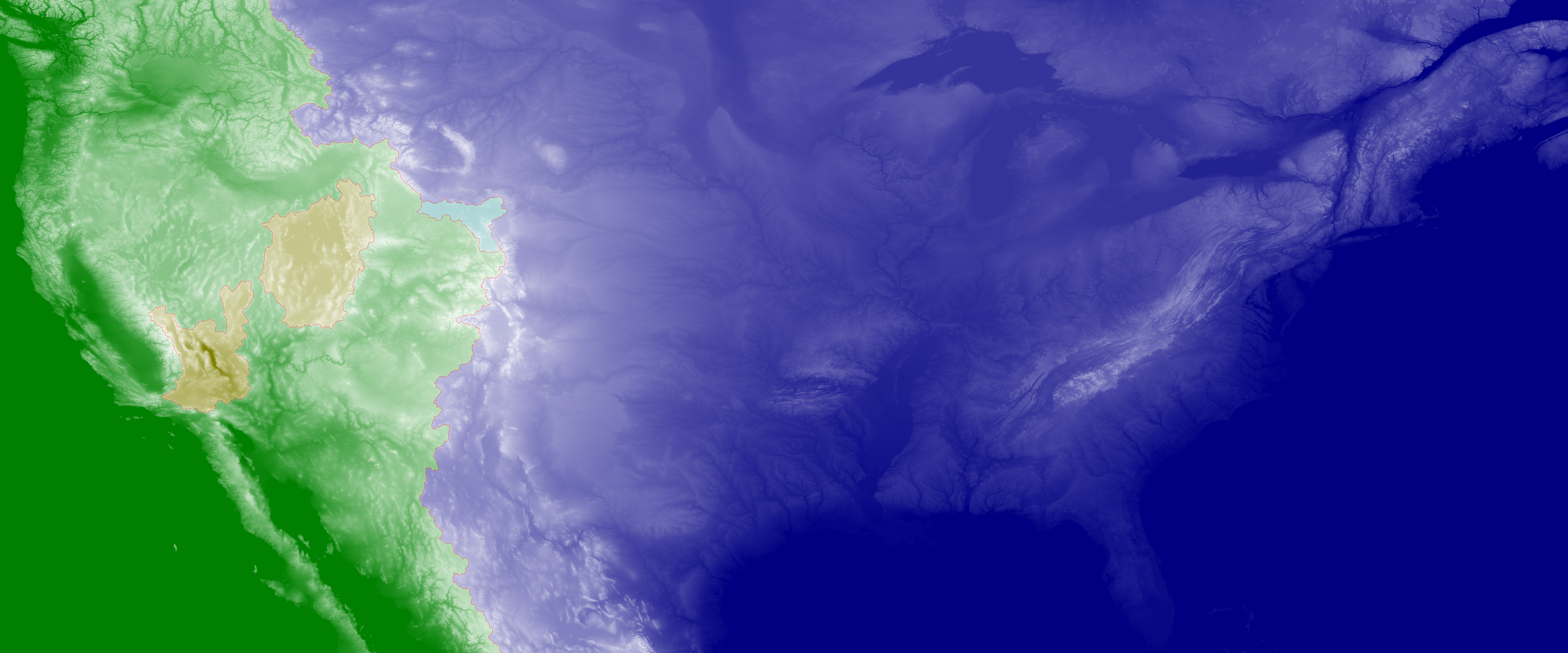
Here’s the answer to that question:
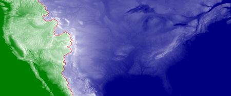
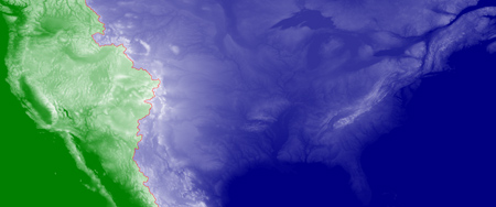
The upper map is the original version from 2000; the lower one uses the 30-arc-second elevation data. The red line is the computed location of the Great Divide, separating the blue Atlantic from the green Pacific. Over most of the length of the divide, the two maps coincide pretty closely, but there’s a notable deviation in western Wyoming, just above the middle latitude of the region shown. On the low-res map, the Atlantic bulges westward from the Wind River Range all the way to the Utah border. In the high-res map, the Pacific has reclaimed that territory. Which map is correct? I’ll come back to that question, but first I want to point out that creating the higher-resolution image was not just a matter of dusting off the old program and running it on new data. What fun would that be, anyway?
When the project began in 2000, I was working on a brand new Macintosh G4 running MacOS 9.0.4, and my favorite programming environment was MacGambit, an implementation of the Scheme programming language created by Marc Feeley. By now, my old G4 is probably leaching heavy metals into some Asian landfill, and the software of that era is equally inaccessible. Nevertheless, the divide-drawing program was not beyond salvaging. After an hour of fiddling and tweaking, I got it running on new hardware with a new operating system and a new Scheme implementation. I was able to regenerate the same maps I produced nine years ago, using the same data as input. But working with the higher-resolution terrain models was another matter. A first try with the 30-arc-second data ran for 12 hours without producing a result.
The ETOPO5 map, with its 100-square-kilometer pixels, dices my slice of North America into a 720-by-300 array, for a total of 216,000 pixels. When I downloaded a swath of the GLOBE Database covering the same territory, I had a 7,200-by-3,000 array, or 21.6 megapixels. If we assume that the program’s running time is proportional to the pixel count—that it’s an O(n) program—then we should expect a 100-fold increase. That would be bad enough, but on reviewing the code I got worse news: I discovered that one step in the algorithm was likely to be quadratic in the number of pixels—O(n2) rather than O(n). That meant a 10,000-fold increase in running time.
Here’s the basic idea behind the divide-finding algorithm. You start by putting a drop of blue dye somewhere in the Atlantic and a drop of green dye in the Pacific. Then you gradually raise the water level, letting each ocean flood the adjacent shoreline pixel by pixel. (I named the main procedure global-warming.) Eventually, the blue and green waters have to meet; where they do, erect a red wall to keep them from mixing. As the waters continue to rise, extend the wall as needed. The path of the red wall is the continental divide. A simple invariant captures the essence of this process: A pixel p is on the divide if and only if, at some point in the process of raising the sea level, p is still unflooded but has neighboring pixels of different colors.
A crucial requirement of the algorithm is that the two oceans rise synchronously; otherwise, one ocean would reach the site of the divide first and would spill over into the other basin. In a physical model (i.e., real water) you could count on the self-leveling property of liquids to enforce the rule of simultaneity; but computational fluids are not so cooperative. To avoid spillage, I raised the level of each ocean in small increments, equal to the difference in elevation between the current water level and the height of the next highest pixel anywhere in the terrain. To implement this idea, I set up a baroquely complicated structure of stacks and queues, which kept track of all pixels currently at the land-water interface. That’s where the quadratic process intruded. I was adding each neighbor of each coastline pixel to a linked list, and checking in each case that the neighbor wasn’t already present in the list. Checking for uniqueness in an unordered list of n items takes n steps, and performing the check for each of the n items therefore takes n2 steps.
(Actually, the n in this formula is not the total number of pixels in the map. It’s the number of pixels on the waterline. How large could a list of waterline pixels grow? The length of the list is given by the fractal dimension of the coastline! That dimension is likely to be somewhere near 1.5. For the 7,200-by-3,000-pixel map, we can expect roughly 300,000 pixels in the list. Thus the situation isn’t quite as bleak as 21,600,0002, but the square of 300,000 is still a large number; I don’t want to have to do anything 300,0002 times.)
There are lots of remedies for this problem—a sorted list, a priority queue, a hash table. I wound up taking a really easy way out: I just ignored the problem. It’s much quicker to store a pixel twice and then discard the duplicate than it is to check in advance for uniqueness. No pixel can appear in the queue more than four times (once for each neighbor), and so the cost in wasted space is tolerable. The data structure I finally settled on is an array of stacks, with one stack for each elevation in the map. (There are roughly 4,000 distinct elevations, measured in integer units of one meter.) Pushing a pixel onto a stack is an O(1) operation. Popping a pixel off the array of stacks is usually O(1) as well, although there’s an additional small cost when we take the last pixel at a given elevation and have to search for the next occupied level.
When Bill Casselman proposed the Notices cover, I set out merely to revise and tidy up my old program, but inevitably I succumbed to the urge to scrap it all and start fresh. The new program is written in Common Lisp rather than Scheme—not for any deep reason, just because that’s the flavor of the week. The new version sifts through the 21-megapixel map in a matter of seconds, although writing out Postscript images at various stages in the process (125 megabytes each) takes somewhat longer.
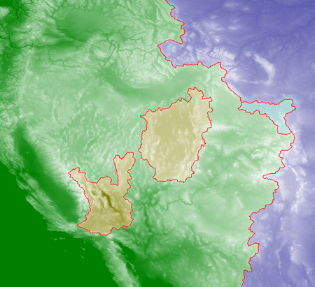
So what about that Wyoming bulge? When I first noticed the discrepancy between the older and the newer maps, I thought I knew exactly what was going on. Some diagrams of the continental divide show a “bubble” in Wyoming, where the divide itself divides, and then the two branches rejoin, enclosing a basin that doesn’t drain into either ocean. I immediately guessed that my program was following one edge of the bubble with the low-resolution data and taking the other path with the high-res data. But that’s not the answer. The bulge is too large and in the wrong place. Here are details extracted from the two maps (one has been enlarged and the other reduced):
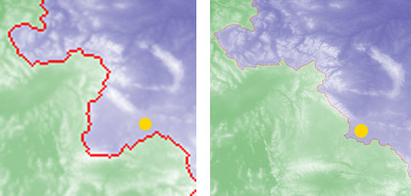
The bubble, if it exists, is roughly in the position of the yellow dot, southeast of the prominent white “eyebrow” formed by the Wind River Range. In the low-res map, the divide takes an excursion 150 kilometers farther west, circling another major basin. I’ve seen no published sources that support this geography; all maps show the divide following the Wind River Range, as in the high-res image at right above. River drainage patterns on standard maps also make it clear: Streams on the western slopes of the Wind River Range flow into the Green River and then into the Colorado. Thus if you make a rest stop at Marbleton, Wyoming, near the center of these images, what you leave behind will end up in the Pacific, not the Atlantic. And so I have to conclude that my 2000 map of the divide, which has now been published three times (in American Scientist, in Group Theory in the Bedroom and on the cover of the Notices), takes us down the wrong path in this region.
The cause of the error could be a bug in my program—it wouldn’t be the first time—but I don’t think that’s what’s going on here. I believe that both maps correctly describe drainage patterns on the landscapes they represent, but those landscapes are not the real North American continent; they are checkerboard arrays of absolutely level, absolutely square tiles. Smaller tiles capture more detail than large ones. In particular, the 100-square-kilometer tiles of the ETOPO5 map flatten out small topographic features that might form a barrier to the flow of water. With closer scrutiny, perhaps I’ll be able to identify the specific site of the leak.
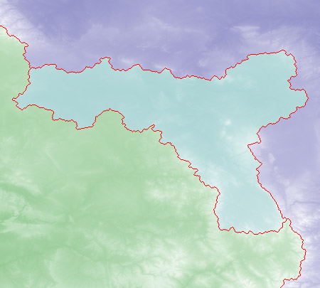
Interestingly, the “bubble” explanation that I hoped would account for differences between the 5-minute and the 30-second maps does appear to work in the case of the 1-minute and the 30-second maps. The image below superimposes the divides calculated by the algorithm for these two data sets, with the 1-minute map in blue and the 30-second map in red:
The paths diverge just southeast of the Wind River Range, forming a bubble very much like the one on standard topo maps. There’s another smaller bubble to the northwest, in the Yellowstone caldera. Everywhere else, the two trajectories agree to within a pixel or two.
If the Wind River bubble is a real feature of the North American landscape, shouldn’t a divide-finding program detect it? In the global-warming algorithm, if you start out by dyeing one pixel blue and another green, you are guaranteed to get a two-coloring of the entire map. The expansion of one color cannot stop until it butts up against the other color; there’s no way to leave an uncolored void. The series of diagrams below shows what happens.
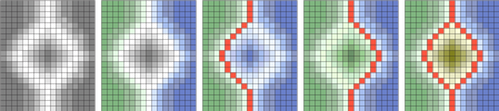
At the far left is the initial state: a ridge with a bubble in the middle. In the second panel, the blue and green waters are lapping at the rim of the central basin. The barrier is perfectly symmetrical, with all pixels on the rim at the same height. Nevertheless, the symmetry is necessarily broken when the sea level is raised still further. The basin is filled either with blue or with green, and the divide runs only on one side; the result looks like either the third or the fourth panel. The choice is essentially random, determined by the sequence in which the pixels are flooded. The only way to create a bubble in the divide is to deliberately implant a seed for a third color in the interior of the basin, as shown at the far right.
The 2000 version of the program was hard-wired for two colors only. It knew about the Atlantic and the Pacific but had no provisions for other bodies of water. In the rewrite I allowed for additional basins. Below is a detail of a high-resolution map seeded to create independent watersheds in the Wyoming bubble and also in two other basins that don’t currently have significant natural drainage to an ocean.
Here’s the computed outline of the bubble at 100 percent magnification:
It looks plausible enough, but I need to add a caveat: Just as the two-color version of the program is certain to produce a two-colored map, starting with three colors ensures that the map will show three watersheds, whether or not they exist on the landscape. For that bubble to be a real feature, under the strictest definition of a divide, the two branches of the divide must have the same minimum elevation. If two hikers walked along those paths, each carrying an instrument that records their minimum altitude, the readings would match when they reunited. The fact that the flooding algorithm shows a bubble in the divide does not guarantee that this condition is satisfied. Seeding a third color anywhere on the map will produce a basin of that color.
Quite apart from the whole question of continental divides and mathematical analysis of terrain, I have become enchanted by the ghostly view of landforms that emerges from a simple grayscale rendering of the high-resolution elevation maps.
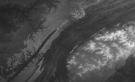
Above is a region of southern Appalachia, where the feathery dendritic traces of drainage channels seem to be inscribed as positive images in some areas and negatives elsewhere.
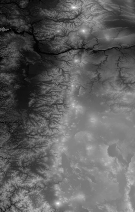
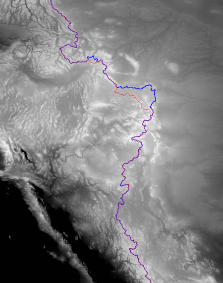
On the west coast (above), we see more dramatic drainage patterns (the big river near the top is the Columbia) and also a glorious string of volcanoes lit up like a constellation in the night sky, from Mount Shasta at the bottom to the diamond configuration of Mount Hood, Mount St. Helens, Mount Adams and Mount Rainier at the top.
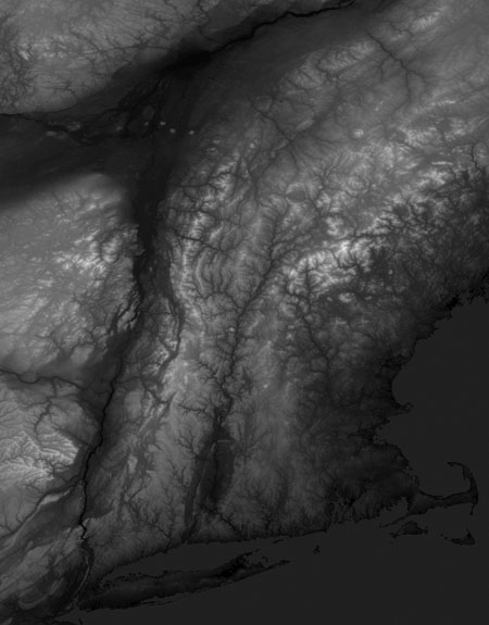
Finally there’s this disturbing image. I don’t think I would be able to identify the location if it weren’t for the telltale forms of Long Island and Cape Cod toward the bottom. The deep north-to-south fissure at the left is the Hudson River Valley; the even bigger diagonal gash at the top is the St. Lawrence. Together they cut off the New England states and the Atlantic provinces of Canada, which seem not to belong to the same continent as the rest of us. What we’re seeing here looks for all the world like a great mass of bedrock scraped clean by glacial action, but remember that this is not a photographic image or anything like one; it’s an elevation map. Most of what looks like polished bare rock is actually forested terrain.
Also intriguing is a line of white dots—they look like puffs of smoke—in the St. Lawrence valley. I thought at first they must be some artifact in the data, but a glance at satellite photos shows they’re quite real. They are the Monteregian Hills, isolated outcroppings of igneous (but not volcanic) rock exposed as softer surrounding material has washed away. One of the dots is Mont-Royal, the hill from which Montreal takes its name.
All these features are best appreciated in the full, high-resolution images. Frustratingly, I can’t show those here. I’m sure I’ve already transgressed on the bounds of blog politeness with this long and bulky post; adding a 125-megabyte image file would get me beaten up by the bandwidth bullies. The best I can offer is a pair of images that are full size in terms of pixel count (7,200 by 3,000) but have been JPEG compressed to a more manageable size. Click to download the unadorned 30-arc-second base map (1.2 MB) or the final continental-divide diagram, with bubbles and extra basins (1.8 MB). Almost forgot: There’s also an animated GIF that I did back in 2000. And if anyone wants it, I can post the Lisp source code.
There’s still more that might be done on the theme of continental divides. One project I have in mind is to add the rest of North America. I hear there’s a whole nother country up there beyond the 49th parallel, with drainage into the Arctic Ocean.
Update 2009-02-11: Thanks to all those who asked about the source code. I’m grateful not only for the interest but also for the nudge to properly document the program, which I would not have done if left to my own devices. Of course I found another bug. (The very last one, surely!) Because of an off-by-one error, the program was ignoring the very highest pixels in the landscape.
Anyway, the source code is now online here.
Quick responses to some of the comments:
Thanks for the tip on the Shuttle Radar Topography Mission data. It looks like a fabulous resource for some project focused on a smaller area, but I’m not quite ready to bump up the data volume by another factor of 900.
Graph cuts for image segmentation: New to me. Evidently I need to do some reading. Thanks for the pointer. (I am aware of connections to other work on image segmentation; this was discussed at the end of my 2000 article.)
The idea of inundating the landscape and then doing the analysis as the water drains away is intriguing, but I can’t see quite how to make it work. At the instant when the first peak of land emerges, the waters extend continuously in every direction. How do you deduce which area drains to which basin? Or am I missing something obvious?
On the problem of demarcating boundaries between oceans: The traditional definition of a topologist is someone who can’t tell a donut from a coffee cup. Now we have a new definition: Someone who goes swimming in Asbury Park and expects to come out of the water in Malibu. Yes, mathematically there’s no clear boundary between the Atlantic and the Pacific; all the waters communicate, and there’s really just one world ocean. But some of us can still tell the difference between New Jersey and California.
Norway: The NGDC data covers the globe, so you should be able to do a Scandinavian map. As for the lake that drains to both coasts, the weirdest geographic fact I know is something I learned from a reader of my American Scientist column: I’m told that you can take a boat up the Orinoco River in Venezuela and without ever leaving the water cross over into the Amazon basin, continuing downstream back to the sea in Brazil. The continental divide is underwater!
To Brooks Moses on the idea of automatically identifying basins: There are some corner cases where you need to be cautious. For example, what happens when the Atlantic and the Pacific both reach the rim of a basin at the same time? Nevertheless, I think you’re right, and a careful implementation of your idea would work as you describe. But is the output useful? In the low-resolution (5 minute) map of the U.S. there are at least 10,000 independent watersheds that your algorithm would identify and color. There would be even more in the high-res data. The spiderweb of divides becomes so dense that you learn nothing about overall drainage patterns. For other applications—especially in image analysis—finding segments without the need for manual seeding is what it’s all about, but the situation is not so clear for the peculiar problem of geographic watersheds.
As the Wikipedia entry on the Great Basin shows, there are at least 72 separate watersheds within it, and the list is doubtless not complete.
Please do post the source, preferably with a permissive Open Source license like new-BSD or Apache 2.0.
The incomparable John McPhee, _Rising from the Plains_ (1986, but I quote from the possibly revised version incorporated in _Annals of the Former World_, 1998):
“West of Rawlins [south central Wyoming] on Interstate 80… a region a good deal flatter than most of Iowa… we passed a sign informing us that we were crossing the Continental Divide. So level is the land there that the divide is somewhat moot. Cartographers seem to have difficulty determining where it is. Its location will vary from map to map. Moreover, it frays, separates, and, like an eye in old rope, surrounds a couple of million acres that do not drain either to the Atlantic or the Pacific — adding ambiguity to the word ‘divide.’”
This is really quite nifty. Thanks for the information on how you calculated the Great Divide. Very cool.
Hasn’t your program just found the Great Divide Basin in central Wyoming?
http://en.wikipedia.org/wiki/Great_Divide_Basin
John, I’ll second the source code request, but I think you’re stuck in a different basin than the one under discussion. The Great Basin is not adjacent to the Continental Divide.
Wow- what a fantastic read. Thank you so much!
I used to be a homeless rodeo clown but now I am a world class magician !
If you really want to get carried away, the Shuttle Radar Topography Mission elevation data is available at http://www2.jpl.nasa.gov/srtm/, and offers 1 arc-second (~30m) resolution over nearly all of the the USA (a few regions occluded from the Shuttle’s view by high mountains are filled from older data), and 3 arc-second worldwide.
Have you thought about using graph cuts to solve this segmentation problem? I think that if you tried setting the weight for each edge according to (MAX_HEIGHT - difference) then you ought to be able to get similar results.
Here is a tutorial: http://www.cis.upenn.edu/~jshi/GraphTutorial/
For the multicolor case, an optimal segmentation can be approximated to within a constant factor of optimality using Boykov & Kolmogorov’s method.
What if you did the reverse process: flood everything, and slowly drain away, checking for the moment when the fluids part? Seems that this would generate the basin boundaries.
Very interesting read. I thoroughly enjoyed it and loved the images. Thanks.
If you wish to do all of North America, you get a problem with definitions: The continental US (excluding Alaska) is handy in that the wet portion of its boundary has two components. For North America there is only one. Where do you say the Atlantic coast stops? Or where the Pacific starts? And should you count the Arctic sea as a separate body of water? Ideally, one should be able to color the coastline with a continuously varying color, then color the whole continent according to where a falling raindrop drains into the sea. But your approach does not seem amenable to dealing with this much harder problem.
Count this as one vote for “release Lisp source.” Fascinating article, as well!
It would indeed be interesting to have the source code. Here in Norway, we have a lake that actually drains into two rivers, one heading west and one heading east. So anything draining into that lake should have a different colour. I am not sure how that could be achieved, but it should be similar to your bubbles. (Not sure if I can get hold of good enough map data.)
It would be difficult to reverse the algorithm to find basins. To decide which point to remove you would want to remove the highest point under a body of water that includes one of the oceans. I don’t see an easy way to tell the difference between a point under water in a basin and a point under water that is connected to an ocean.
The continuously varied coastline sounds like a fun idea, but I expect the results will be very similar to what would happen if you put a seed point wherever a river meets an ocean.
Incidentally, it should be pretty easy to extend the algorithm to find new basins/bubbles, rather than arbitrarily coloring them in with the color of an adjacent basin.
A characteristic of an unseeded basin is that any pixel on its rim drains into an area that has not yet been colored. Thus, when the coloring algorithm reaches the lowest point on the rim, the pixels inside the basin will have the property that they are (a) uncolored, and (b) lower than the current “water level”.
Thus, when you color a pixel, you can add a check to see whether it is in fact in the band of elevations that you are expecting to color. If it is below that level, it must be inside an unseeded basin. Thus, you can follow a steepest-descent algorithm to find the spot at the bottom of the basin, place a seed there, and raise the water level on that seed until it reaches the current level.
We know that the steepest-descent algorithm will do the right thing. It won’t run into an existing basin, because that would require there to be an uncolored pixel that is lower than the one we started with, but which is adjacent to an existing basin; this cannot happen because of the order in which basins are colored. Also, any uncolored pixel that the steepest-descent algorithm lands on will be the bottom of a basin; if steepest-descents from all pixels in an uncolored region do not resolve to a unique answer, that means either that the bottom is flat (so it doesn’t matter) or that there are multiple unseeded basins within the region. The basin-filling algorithm should be recursive; if you find another unseeded basin while doing this, you go and fill it in, and then raise the pair up to the main current level.
A relevant observation is that, since the basin is previously-undiscovered, we know that the filling process will not reach a boundary with the existing basins/oceans until we get up to the current level, and thus the result is not different from having placed seeds in the basins a priori.
Here’s an idea:
put the pixels in a priority queue with lowest-height first.
put each pixel into its own set
for all pixels of the next-lowest height. . .
remove the next pixel and mark it colored. among all of its adjacent, colored, neighbors, choose that with the greatest height (aka the neighbor with best matching height)
if there is such a neighbor (could be NO neighbors are colored), union the sets of the current pixel and its neighbor
repeat the loop until queue is empty.
Sets now contain the terrain, properly divided up.
Simple, n lg n algorithm due to the priority queue. Everything else is linear time.
I think there is a very simple O(n) algorithm. Just start from each pixel in the image and find the fastest way downwards. When you end up at a minimum, mark all pixels traversed with the location of the minimum pixel. Likewise if you run into an already-marked pixel, mark back the current path. Choose a color for each minimum found. Of course you need to put artificial rigdes into the ocean when you do the whole of north america.
Andreas, that algorithm makes quite a bit of sense, and solves some of the problems described above, but I don’t think it’s O(n). That is definitely a lower bound for any algorithm; you have to go to each pixel to color it. For your algorithm, for each pixel you color, you have to traverse some sequence of untraversed pixels. You could probably make an argument that the length of that sequence will decrease at a particular speed, and maybe that would give an O(n log n) or similar complexity.
O(n) with n being the number of pixels in the map, of course. And for each pixel when I build a path to the local minimun or an already-colored pixel, I traverse a path of some number of pixel, but I can color all of them in this iteration. Basically I only need to look at each pixel to or three times — when I try to start from one that is already colored no work is needed.
Because I can truncate the minimum search when I encounter an already-colored pixel, I will search long paths for some pixels, but I will only try to find the steepest descent from each pixel one time — when it is not yet colored.
So far, so bad. My simple algo apparently suffers badly from the noise in the data. I’m using the german area, an my paths seldom reach more than a few pixels before getting stuck somewhere….wait a minute.
Ok, the algorithm at least needs a way to fill plateaus and find an exit from those, just finding a local descent gets stuck in those as well.
Also the raw data (GLOBE) contains some artefacts, in http://ch.iocl.org/g.png (falsecolor to bring out small-elevation features) near the upper left water (pink) there are a few features that are too rectangular to be of natural origin.
As a boater, I found this of interest… I’m not sure why, but :-)
Especially the part about sailing over the continental divide… that just sounds slick.
http://www.craftacraft.com/continental_divide
Pingback: Out of the cesspool and into the sewer: A/B testing trap : Credit Debt Banking News | CDBN