In Zeno’s Footsteps
by Brian Hayes
Published 10 April 2008
The latest issue of American Scientist is just out, both on the newsstand and on the web. My “Computing Science” column is titled “Wagering with Zeno”; it returns to a subject mentioned briefly in an earlier column, “Follow the Money.”
Consider a random walk on the interval (0,1), where the walker moves according to these rules:
- The walker begins at x = 1/2.
- At each step the walker moves either left (toward 0) or right (toward 1) with equal probability.
- The length of each step is one-half the distance to 0 or to 1, whichever is nearer. In other words, the distance moved is 1/2 min(x, 1–x).
If you want to know more about this process and why I bothered to write about it, please see the column. Here I just want to say a few words about visual aids that might be helpful in understanding how the random walk evolves and where the walker is likely to wind up.
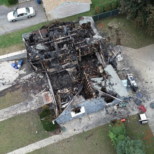
Here is one of the illustrations that appears in the column:

We see four trajectories, each lasting 10 steps. Although the walk is actually one-dimensional—moving back and forth along an interval of the x axis—the trajectories are plotted in two dimensions for clarity, moving down the page so that the illustration becomes a kind of discrete spacetime diagram. Even with this device, though, some of the paths overlap for part of their course. If I tried to crowd more trajectories into the figure, the overlaps would make it hard to sort out one walk from another.
In making pictures like this, the issue is not just how you explain an experiment to other people; it’s also a matter of how you come to understand the process yourself. While I was trying to make sense of the Zeno walk, I plotted lots of trajectories like these, initially by hand and then with a program that generated Postscript files. Some important features were quickly apparent. In particular, I noticed that the walker takes much bigger strides in the middle of the space than near the edges. (Of course this fact follows directly from the definition of the walk, but it doesn’t hurt to see a picture.) I also observed that most of the walks seem to spend most of their time hugging one edge or the other, seldom venturing back across the midline of the space. Even after looking at a few hundred examples, however, I didn’t feel like I had a really secure sense of how a “typical” walk would proceed.
As with many processes that evolve over time, the illustrative possibilities are much richer if we can escape the static bounds of ink on paper. And thus I was led to try creating a more dynamic and interactive display.

What you see above is not dynamic; it’s merely static pixels on glass. But you can see it all in action in this Java applet. Feel free to click on the link and go play, but do come back here afterward so we can continue the conversation.
Hello again.
Does this program succeed in conveying an intuitive sense of how the Zeno walker walks? Personally, I’ve found it helpful, although it still comes up far short of ideal. Adjusting the number of steps in each walk gives a sense of how the walker’s apparent attraction to the edges gets more extreme over time. And adjusting the rate at which paths fade into the background allows for a degree of balance between clutter and evanescence. But there may well be a better way to go about visualizing these concepts. I’d be interested in hearing suggestions.
A note on the implementation: The applet was created with the programming language called Processing, invented by Ben Fry and Casey Reas. I’ve just reviewed two books on Processing, and so this project was undertaken partly to try out the language and its programming environment. I found it very slick, and mostly trouble-free. The source code of the zenowalk program is available through a link on the applet page. (Most of the code for the buttons and sliders was cribbed from the book by Fry and Reas.)
Of course there’s always something lacking in any programming language. In this case what I missed most acutely was the exact rational arithmetic I rely on in Lisp. Processing has only single-precision floating-point numbers. In the Zeno walk, these numbers begin running out of significant digits after about 150 steps (which is why I limited the program to 145 steps). As far as I can tell, no one has yet written a Processing library for bignums and exact rationals. I guess that’s my job.
Responses from readers:
Please note: The bit-player website is no longer equipped to accept and publish comments from readers, but the author is still eager to hear from you. Send comments, criticism, compliments, or corrections to brian@bit-player.org.
Publication history
First publication: 10 April 2008
Converted to Eleventy framework: 22 April 2025


I’ve thought some about the questions in your article.
I prefer a variation where only the numbers between 0 and 1/2 are considered; then we always multiply by either 1/2 or 3/2 (and if multiplying by 3/2 gives a number > 1/2, subtract it from 1 to get a number < 1/2, and record a midline crossing).
In this scenario, we might as well start at level 2, with the number 1/4.
I’ve got some lemmas about the structure of Zeno-tree numbers that lead to a fairly fast algorithm for counting the numbers.
Consider an arbitary Zeno-tree number, like 7/16, and a path through the tree to get to that number (1/4 -> 3/8 -> (midline crossing) 7/16). Label the transitions in this path with either N (no crossing) or C (crossing); then this path gets the label NC. Given such a label ending with a C, there is at most one rational number with a path with that label.
We can prove this by induction. Consider a label L, ending with a C. Remove this C, then remove any trailing N’s from the remainder, to get a path L’; if we removed k N’s, we write this as L = L’ N^k C. Either L’ ends with a C (in which case it has at most one associated rational number), or it is the empty path (in which case it is associated with 1/4). If L’ has no associated rational, then neither does L. If L’ has an associated rational p, then consider the numbers (3^j/2^{k+1})*p, for nonnegative j. If one of these numbers falls between 1/2 and 1, then L is associated with 1-(3^j/2^{k+1))*p; otherwise, L is associated with no rational.
A path L that does not end with a C (so L = L’ N^k) is potentially associated with a set of rationals. Suppose that L’ is associated with the rational p; then L is associated with the set { (3^j/2^k)*p | j ≥ 0 and (3^j/2^k)*p ≤ 1/2 }.
Conversely, each Zeno-tree number is associated with exactly one label. First we note that if a label L ends with a C, then the numerator of its associated rational is not a multiple of 3. (Because the associated rational is 1 - 3n/2^k = (2^k - 3n)/2^k, for some integers n and k; since 3n is a multiple of 3 and 2^k is not, 2^k-3n is also not a multiple of 3.)
Suppose that some Zeno-tree number is reachable by two paths with different labels. Pick such a number p of lowest level, and consider the labels L1 and L2 of paths that reach this number. These labels must be the same length, since the length of the label determines the denominator of the number. The numerator of p must not be a multiple of 3; if it were, then both labels must end with at least one N, and p/(3/2) would be a number of lower level with two distinct labels.
Now if both labels end with N, then p/(1/2) (= 2*p) is a number of lower level with two distinct labels; and if both labels end with C, then (1-p)/(3/2) is a number of lower level with two distinct labels. The remaining case is that one label ends with N and the other ends with C, where the N represents a division by 2. Call p’s parent on the N-path p1, and on the C-path p2; then p = p1/2 = 1-(3*p2/2). But we know that p1 < 1/2, which gives us that p < 1/4; and we know that p2 < 1/2, which gives us that p > 1/4; so this case is also impossible. (This is why we start with stage 2; if we started with the number 1/2 in stage 1, then the path N and C both lead to 1/4.)
So each Zeno-tree number has at most one label, and each label corresponds to a computable set of numbers. Then we can study the set of numbers by studying the set of valid labels.
In particular, this gives us a way to enumerate the Zeno-tree numbers of a given level without explicitly checking for duplicates. I’ve written a Sage function to do this enumeration; for each label, it keeps track of the largest numerator of a number with that label. (It does not store the labels at all, only the numbers.) At each level, the set of Zeno-tree numerators is the union of two disjoint sets: the set of numerators from the previous level (which I do not explicitly keep; I only keep a count of them) and the numerators that you get by taking the “largest numerator” set mentioned before and multiplying by 3/2 (and subtracting from 1, if the new number is > 1/2).
If you have a copy of Sage, you can run this by typing:
sage: load http://sage.math.washington.edu/home/cwitty/zeno.py
sage: count_zeno_numbers()
With a lot of patience (and a machine with at least 5 gigabytes of memory), this will tell you, for instance, that level 51 has 146757015 Zeno-tree numbers between 0 and 1/2 (or 293514030 between 0 and 1); this is a density of 146757015/562949953421312, or 2.6 * 10^{-7}, which is 0.723286 times the density of level 50. (The ratios of densities between successive levels seem to converge to approximately 0.7233.)
By the way, there seems to be an error in the article; it gives the density for level 9 as 25/128, but according to two separate programs I’ve written, the true answer is 26/128 (= 13/64).
This gives strong confirming evidence that the density does go to 0 as the level increases (although, of course, it is not a proof).
For the third question, at any point in the game, the probability of a subsequent midline crossing is greater than zero; perhaps a more interesting question is whether the expected number of subsequent midline crossings is finite or infinite.
I really wish your blog comments had “preview”!
Many thanks to Carl Witty for incisive analysis. A few quick comments on the comment:
1. Witty is correct about the error in the article. Simple careless counting on my part.
2. The “folded” version of the walk, confined to the interval between 0 and 1/2, is indeed convenient for computations. I avoided mentioning it in the article because it’s not so convenient for exposition.
3. “… a more interesting question is whether the expected number of subsequent midline crossings is finite or infinite.” Witty has said exactly what I should have said in the article. This is indeed the right question.
4. I too wish my blog comments had “preview.” I’ll see what I can do.
Great problem, and a great column. I’d like to share some thoughts on the density of Zeno tree numbers.
Let f(n) be the number of distinct Zeno-tree numbers after n rounds, where round n is the one in which all of the outcomes have 2^(n+1) in their denominator. As the bar chart in the article reveals, f(1)=2, f(2)=4, f(3)=6, f(4)=10, f(5)=16. Brian conjectures that f(n)/2^n -> 0, i.e. the density of Zeno-tree outcomes in the dyadic rationals goes to zero. I think this can be proven as follows (this is just a game plan, and the proofs are conspicuously absent).
Let d(n) be the number of outcomes in round n that are less than 1/2 and that share a child with another, larger outcome in round n. For example, in round 4, the outcome 1/32 is such an outcome, because one of its children is 3/64 which is also the child of 3/32. Similarly 3/32 is itself such an outcome since it shares the child 9/64 with 9/32. The outcome 9/32, however, is not such an outcome, so we have d(4)=2. In fact it’s easy to read off d(1)=0, d(2)=d(3)=1 and also d(5)=4.
Brian’s data strongly suggest the following.
Conjecture: An outcome in round n+1 is the child of at most two outcomes in round n.
This conjecture immediately implies the recurrence relation
f(n) = 2 ( f(n-1) - d(n-1) )
because the number of children in round n is twice the number of parents f(n-1), minus the number of parents that share a child with some other, larger parent, which is d(n-1) in the interval (0,1/2) and hence 2d(n-1) by symmetry. The data above satisfy this equation.
Which outcomes get counted in d(n)? Consulting the data in the article, it really looks like two outcomes a/2^n and b/2^n share a child only when they are “adjacent” powers of 3. Thus the data strongly suggest the following (here I use the random walk terminology).
Conjecture: If a/2^n and b/2^n are outcomes in round n (with a less than b less than 1/2) such that stepping right from a/2^n and stepping left from b/2^n yields the same outcome, then a=3^k and b=3^{k+1} for some k.
This conjecture then implies that d(n) is precisely equal to one less than the number of dyadic rationals less than 1/2 and of the form 3^k/2^n for some k (one less because the last one doesn’t count), and this quantity is just the floor of n/log_2(3) modulo some constants.
If we conjecture this explicit form for d(n), it should be possible to solve the recurrence above and get an explicit formula for f(n). I tried doing this with generating functions, but it gets very messy; maybe there’s some kind of general result that can be applied in this case.
My guess is that the solution would reveal that f(n)=O(s^n) for some s less than 2, which would then imply that f(n)/2^n goes to 0 as conjectured (Carl Witty’s experiments suggest what we can expect s to be).
It is true that a/2^n and b/2^n share a child only if b/a = 3, but it is not true that a and b must be powers of 3. The smallest counterexample is 7/64 and 21/64, which share the child 21/128.
Carl, you’re very clearly right, so there are more repeated children than I thought. This is probably good, since it suggests that it’s possible to deduce an even larger lower bound for d(n), and then, as before, use it with the recurrence
f(n) = 2 ( f(n-1) - d(n-1) )
to give an even lower upper bound on f(n).
I went back and read “Follow the Moneyâ€, and it seemed that an enterprising undergraduate could leaven in some “Evolution of Cooperation” ideas to see if trading oligarchies develop.
Hello Brian;
I’ve enjoyed your articles over the past years. So I was happy to see you ask a question in your column that allowed me to send you an email. I’ve been teaching Markov chains to undergrads and have been pushing martingales. So I will be assigning your article for the next homework as a reading. I’ll see if I can walk them through answering your 3rd question.
You describe a gambling game with dyadic pay-outs. The key thing is that you keep it fair, so the wealth is a martingale. Further you keep it bounded. So via a nuclear strike theorem, we can answer the 3rd question. The theorem says (in one of its many forms):
If X_t is a bounded martingale, then X_t converges to X_\infty almost
surely.
(Pardon my latex.)
So we know that X_t will stay within an epsilon neighborhood of some point which we can call X_\infty. So it will cross at most a finite number of times.
This is kinda useless as a result since it tells us little about the finite case nor does it provide much motivation as to why it is going on. So the correct result to use is the following:
If X_t is a martingale that is never negative, then
P(Max X_s > M) < X_0/M
This is called the martingale maximal inequality. It is totally amazing and useful. The one line proof goes as follows. Stop the martingale the first time it is bigger than M. By the optional sampling theorem (i.e. that there is no way to win at a fair game) the expected value of X when you stop it is equal to the initial value. Now doing a bit of math says that the probability of ever being larger than M has the desired bound.
So for the problem that you ask, we can start doing the analysis the first time one of the players has wealth less than epsilon. Then let M=1-epsilon. So the probability that it ever comes to pass that currently “poor” player has wealth greater than 1-epsilon is less than epsilon / (1-epsilon). So we can then say that the chance of one player being reduced to epsilon followed by the other player being reduced to epsilon and then back, for a total of say k repetitions, is less than epsilon^k/(1-epsilon)^k. This falls off very fast as you noticed.
p.s. Here is a potential interesting problem for you to consider computing. You can solve the function
integral pi(x) P(x–>y) = pi(y)
for a function pi(x). This is a stable law. In this problem, it will unfortunately integrate out to infinity–but that isn’t the issue I want to focus on. Using this pi() you can then simulate this process in reverse by assuming the previous round came from the stable distribution. I always find this reverse kinda fun to think about.