My new office space suffers from a shortage of photons, so I’ve been wiring up light fixtures. As I was snaking 14-gauge cable through the ceiling cavity, I began to wonder: 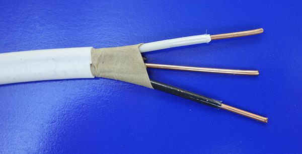 Why is it called 14-gauge? I know that the gauge specifies the size of the copper conductors, but how exactly? The number can’t be a simple measure of diameter or cross-sectional area, because thicker wires have smaller gauge numbers. Twelve-gauge is heavier than 14-gauge, and 10-gauge is even beefier. Going in the other direction, larger numbers denote skinnier wires: 20-gauge for doorbells and thermostats, 24-gauge for telephone wiring.
Why do the numbers run backwards? Could there be a connection with shotguns, whose sizes also seem to go the wrong way? A 20-gauge shotgun has a smaller bore than a 12-gauge, which in turn is smaller than a 10-gauge gun. Mere coincidence?
Answers are not hard to find. The Wikipedia article on American Wire Gauge (AWG) is a good place to start. And there’s a surprising bit of mathematical fun along the way. It turns out that American wire sizes make essential use of the 39th root of 92, a somewhat frillier number than I would have expected to find in this workaday, blue-collar context.
Wire is made by pulling a metal rod through a die—a block of hard material with a hole in it. In cross section, the hole is shaped something like a rocket nozzle, with conical walls that taper down to a narrow throat.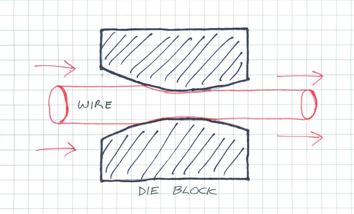 As the rod passes through the die, the metal deforms plastically, reducing the diameter while increasing the length. But there’s a limit to this squeezing and stretching; you can’t transform a short, fat rod into a long, thin wire all in one go. On each pass through a die, the diameter is only slightly reduced—maybe by 10 percent or so. To make a fine wire, you need to shrink the thickness in stages, drawing the wire through several dies in succession. And therein lies the key to wire gauge numbers: The gauge of a wire is the number of dies it must pass through to reach its final diameter. Zero-gauge is the thickness of the original rod, without any drawing operations. Fourteen-gauge wire has been pulled through 14 dies in series.
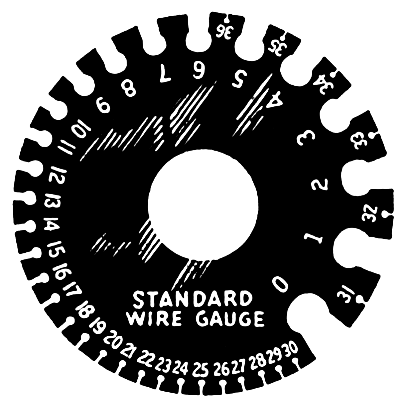
Or at least that was how it worked back when wire-drawing was a hand craft, and nobody worried too much about exact specifications. If two wires had both been pulled through 14 dies, they would both be labeled 14-gauge, but they might well have different diameters if the dies were not identical. By the middle of the 19th century this sort of variation was becoming troublesome; it was time to adopt some standards.
The AWG standard keeps the traditional sequence of gauge numbers but changes their meaning. The gauge is no longer a count of drawing operations; instead each gauge number corresponds to a specific wire diameter. Even so, there’s an effort to keep the new standardized sizes reasonably close to what they were under the old die-counting system.
.png)
The wire-drawing process itself suggests how to do this. Each pass through a die reduces the wire diameter to some fraction of its former size, but the value of the fraction might vary a little from one die to the next. The standard simply decrees that the fraction is exactly the same in all cases. In other words, for every pair of adjacent gauge numbers, the corresponding wire diameters have the same ratio, \(R\).
What remains is to work out the value of \(R\). If we start with \(d_{36} = 0.005\) and multiply by \(R\), we’ll get \(d_{35}\); then, multiplying \(d_{35}\) by \(R\) yields \(d_{34}\), and so on. Continuing in this way, after multiplying by \(R\) \(39\) times, we should arrive at \(d_{-3} = 0.46.\) This iterative process can be summarized as:
\[\frac{d_{-3}}{d_{36}} = R^{39}.\]
Filling in the numeric values, we get:
\[\frac{0.46}{0.005} = 92 = R^{39}, \quad \textrm{and thus}\quad R = \sqrt[39]{92}.\]
And there the number lies before us, the \(39\)th root of \(92\). The numerical value is about \(1.122932\), with \(1/R \approx 0.890526\).
With this fact in hand we can now write down a formula that gives the AWG gauge number \(G\) as a function of wire diameter \(d\) in inches:
\[G(d) = -39 \log_{92} \frac{d}{0.005} + 36.\]
That’s a fairly bizarre-looking formula, with base-92 logarithms and a bunch of arbitrary constants floating around. On the other hand, at least it’s a genuine mathematical function, with a domain covering all the positive real numbers. It’s also smooth and invertible. That’s more than you can say for some other standards, such as the British Imperial Wire Gauge, which pastes together several piecewise linear segments.
Who came up with the rule of \(\sqrt[39]{92}\)? As far as I can tell it was Lucian Sharpe, of Brown and Sharpe, a maker of precision instruments and machine tools in Providence, Rhode Island. A history of the company published in 1949 gives this account:
Another activity begun in the [1850s] was the production of accurate gages. The brass business of Connecticut, centered in the Naugatuck Valley, required sheet metal and wire gauges for measuring their products. Mr. Sharpe, with his methodical mind, conceived the idea of producing sizes of wire in a regular progression, choosing a geometric series as best adapted to these needs. Such gages as were in use prior to this time were the product of English manufacture and were very irregular in their sizes.
The first Brown and Sharpe wire gauge was produced in 1857 and later became the basis of an American standard, which is now administered by ASTM.
Wire gauges are not the only numbers defined by a weird-and-wonderful root-taking procedure. The equal-tempered scale of music theory is based on the 12th root of 2. A musical octave represents a doubling of frequency, and the scale divides this interval into 12 semitones. In the equal-tempered version of the scale, any two adjacent semitones differ by a ratio of \(\sqrt[12]{2}\), or about \(1.05946\). It’s worth noting that instruments were being tuned to this scale well before the invention of logarithms. I assume it was done by ear or perhaps by geometry, not by algebra. Around 1600 Simon Stevin did attempt to calculate numerical values for the pitch intervals by decomposing 12th roots into combinations of square and cube roots; his results were not flawless. What would he have done with 39th roots?
Another example of a backward-running logarithmic progression is the magnitude scale for the brightness of stars and other celestial objects. For the astronomers, the magic number is the fifth root of \(100\), or about \(2.511886\); if two stars differ by one unit of magnitude, this is their brightness ratio. A difference of five magnitudes therefore works out to a hundredfold brightness ratio. Brighter bodies have smaller magnitudes. The star Vega defines magnitude \(0\); the sun has magnitude \(-27\); the faintest stars visible without a telescope are at magnitude \(6\) or \(7\).
The idea of stellar magnitudes is ancient, but the numerical scheme in current use was developed by the British/Indian astronomer N. R. Pogson in 1856. That was just a year before Sharpe came up with his wire gauge scale. Could there be a connection? It would make a nice story if we could find some timely account of Pogson’s work that Sharpe might plausibly have read (maybe in Scientific American, founded 1845), but that’s a pure flight of fancy for now.
And what about those shotguns? Are their gauges also governed by some sort of logarithmic law? No, the numerical similarity of gauges for wires and shotguns really is nothing but coincidence. The shotgun law is not logarithmic but reciprocal. Wikipedia explains:
The gauge of a firearm is a unit of measurement used to express the diameter of the barrel. Gauge is determined from the weight of a solid sphere of lead that will fit the bore of the firearm, and is expressed as the multiplicative inverse of the sphere’s weight as a fraction of a pound, e.g., a one-twelfth pound ball fits a 12-gauge bore. Thus there are twelve 12-gauge balls per pound, etc. The term is related to the measurement of cannon, which were also measured by the weight of their iron round shot; an 8 pounder would fire an 8 lb (3.6 kg) ball.
Addendum 2016-08-08: Leon Harkleroad has brought to my attention his excellent article on “Tuning with Triangles” (College Mathematics Journal, Vol. 39, No. 5 (Nov. 2008), pp. 367–373). He describes a simple geometric procedure that Vincenzo Galilei (father of Galileo) used for fretting stringed instruments. In essence it takes \(18/17 \approx 1.05882\) as an approximation to \(\sqrt[12]{2} \approx 1.05946\).