My column in the new issue of American Scientist is about the challenges of computing with very large numbers. The column ends with an open question, which I want to restate here as an invitation to commentary.
Any system of arithmetic in which numbers occupy a fixed amount of space can accommodate only a finite set of numbers. For example, if all numbers have to fit into a 32-bit register, then there are only 232 representable numbers. So here’s the question: If our numbering system can represent only 4,294,967,296 distinct values, which 4,294,967,296 values should we choose to represent?
There is an obvious trade-off here between range and precision: To reach farther out on the number line, we have to leave wider gaps between successive representable numbers. But that’s not the only choice to be made. We must also decide whether to sprinkle the numbers uniformly across the available range or to pack them densely in some regions while spreading them thinly elsewhere. I’m not at all sure what principles to adopt in trying to identify the best distribution of numbers.
To frame the question more clearly, I’d like to introduce a series of toy number systems. In each of these systems a number is represented by a block of six bits. There are 26=64 possible six-bit patterns, and so there can be no more than 64 distinct numbers. A function f(x) maps each bit pattern x to a number. Sometimes it’s convenient to regard the bit patterns themselves as numbers, ordered in the obvious way, in which case f(x) is a function from numbers to numbers.
In the simplest case, f(x) is just the identity function, and so the bit patterns from 000000 through 111111 map into the counting numbers from 0 through 63. A slightly more general scheme allows f(x) to be a linear transformation, f(x)=ax+b, where the parameters a and b are constants. If a=1 and b=0 we again get the nonnegative counting numbers. If a=1 and b=–32, we have a range of integers from –32 to +31. With a=1/64 and b=0, the entire spectrum of numbers is packed into the interval [0,1). Numbers formed in this way are called fixed-point numbers, since there’s an implied radix point at the same position in all the numbers. By adjusting the values of a and b, we can generate fixed-point numbers to cover any range, but they are always distributed uniformly across that range.
The well-known floating-point number system, modeled on scientific notation, is a tad more complicated. In my toy version, three bits are allocated to an exponent t, which therefore ranges from 0 to 7. The other three bits specify a fractional significand s, interpreted as having values in the range 8/16, 9/16, 10/16, …, 15/16. The mapping function is defined as f(t, s)=s×2t. The 64 numbers generated in this way range from 1/2 to 120. (Real floating-point systems, such as those defined by the IEEE standard, not only have more bits but also have a more elaborate structure, with allowance for positive and negative significands and exponents and various other doodads.)
Floating-point numbers are not distributed uniformly; they are densest at the bottom of their range and grow sparse toward the outskirts of the number line. Specifically, the density of binary floating-point numbers is reduced by half at every integer power of 2. In the toy model, the gap between successive representable numbers is 1/16 in the range between 1/2 and 1, then 1/8 between 1 and 2, then 1/4 between 2 and 4, and so on. At the top of the range—beyond 64—the only numbers that exist are those divisible by 8.
The distribution of floating-point numbers describes a piecewise-linear curve, which approximates the function 2x. In other words, if you squint and turn your head sideways, you can see that floating-point numbers look a lot like base-2 logarithms. This suggests another numbering scheme: Instead of approximating logarithms, why not use the real thing? We can simply interpret a binary pattern as a logarithm and generate numbers by exponentiating. For the six-bit model, we can take the first two bits as the integer part of the logarithm (the characteristic) and the last four bits as the fractional part (the mantissa). Assuming we continue to work in base 2, the number-defining function is just f(x)=2x. The resulting system of six-bit numbers has a range from 1 to about 235. (By simple rescaling, we could make the range of these logarithmic numbers match that of the floating-point numbers, 1/2 to 120. I’ve not done so for a trivial reason: So that in the graphs presented below the two curves do not overlap and obscure each other.)
Finally, I want to mention a fourth numbering scheme, called the level-index system. Indeed, what led me to this whole topic in the first place was an encounter with some papers on level-index numbering written in the 1980s by Charles W. Clenshaw and Frank W. J. Olver. The level-index system takes a step beyond logarithms to iterated logarithms and beyond exponents to towers of exponents. The idea is easiest to explain in terms of the mapping function f(x). As with logarithmic numbers, we view the bit pattern x as the concatenation of an integer part (the level) and a fractional part (the index). Then f(x) takes the following recursive form:
![]()
For any level greater than 0, this formula gives rise to a tower of exponentiations. For example, the level-index number 3.25 expands as follows:
![]()
In the six-bit model, we can dedicate two bits to the integer level and four bits to the fractional index. The result is a numbering system that covers a very wide range: from 0 to almost 400,000 in 64 steps. The distribution of representable numbers in this range is extremely nonuniform: the gap between the two smallest numbers is 1/16, whereas that between the largest numbers is more than 320,000. (Note also that we have shifted from powers to 2 to powers of e. Actually, a level-index system could be defined on any base, but e has some pleasant properties.)
The graph below compares the distribution of numbers in the four six-bit systems.
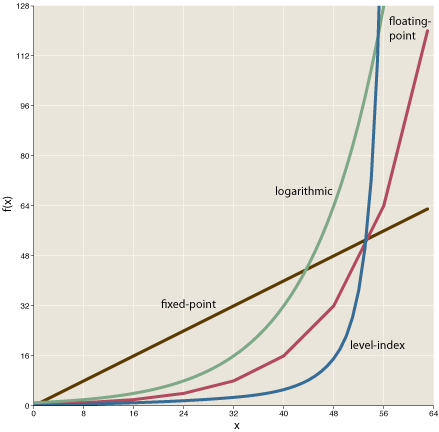
For fixed-point numbers the graph is necessarily a straight line, since the numbers are distributed at equal intervals. The floating-point graph is a jointed sequence of straight-line segments, with the slope doubling at every power of 2. The logarithmic numbers produce a smooth curve, concave-upward. (Again, this curve could be made to coincide with that of the floating-point numbers.) The level-index curve is also smooth but has an even more pronounced elbow or hockey-stick form.
Plotting the same data on log-linear scales clarifies certain details:
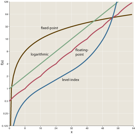
Now it’s the logarithmic system that yields a straight-line graph. The floating-point curve approximates a parallel straight line. The fixed-point graph is concave-downward, while the level-index curve is sigmoid.
By twiddling various knobs and dials, we could create a number system that would approximate any monotonic line or curve in this space, giving us fine-grained control over the distribution of numbers. For example, on the semilogarithmic graph a straight line of any positive slope can be generated by adjusting the base of the logarithmic number system or the radix of a floating-point system; a larger base or radix yields a steeper slope. The inflection of the level-index curve can be altered in the same way, by choosing different bases. If we wished, we could interpolate between the fixed-point curve and the logarithmic curve by creating number systems in which f(x) is some polynomial, such as x2. If we wanted a flatter curve than the fixed-point system, we could build numbers around a function such as f(x)=√2.
So many ways of counting! Let me count the ways.
And so I return to the main question. On what basis should we choose a number system for a digital computer? Let’s leave aside practicalities of implementation: Suppose we could do arithmetic with equal efficiency using any of these schemes. Which of the curves should we prefer? There are plausible arguments for allocating a greater share of our numerical resources to smaller numbers, on the grounds that we spend most of our time on that part of the number line—it’s like the middle-C octave on the piano keyboard. That would seem to favor the logarithmic or floating-point system over fixed-point numbers. But can we make the argument quantitative, so that it will tell us the ideal slope for the logarithmic line, and hence the mathematically optimal base or radix? (Does Benford’s law help at all in making such a decision?)
And what about the level-index system, which skews the distribution even further, providing higher resolution in the neighborhood of 1 in exchange for a sparser population out in the boondocks? An argument in favor of this strategy is that overflow is a more serious failure than loss of precision; the choice is between a less-accurate answer and no answer at all. Level-index numbers grow so fast that they can effectively eliminate overflow: Although it’s a finite system, you can’t fall off the end of the number line.
Some years ago Nick Trefethen, a numerical analyst, wrote down some predictions for the future of scientific computing, including these remarks:
One thing that I believe will last is floating point arithmetic. Of course, the details will change, and in particular, word lengths will continue their progression from 16 to 32 to 64 to 128 bits and beyond…. But I believe the two defining features of floating point arithmetic will persist: relative rather than absolute magnitudes, and rounding of all intermediate quantities. Outside the numerical community, some people feel that floating point arithmetic is an anachronism, a 1950s kludge that is destined to be cast aside as machines become more sophisticated. Computers may have been born as number crunchers, the feeling goes, but now that they are fast enough to do arbitrary symbolic manipulations, we must move to a higher plane. In truth, however, no amount of computer power will change the fact that most numerical problems cannot be solved symbolically. You have to make approximations, and floating-point arithmetic is the best general-purpose approximation idea ever devised.
At this point, predicting the continued survival of floating-point formats seems like a safe bet, if only because of the QWERTY factor—the system is deeply entrenched, and any replacement would have to overcome a great deal of inertia. But Trefethen’s “two defining features of floating point arithmetic” are not actually unique to the floating-point system; logarithmic and level-index numbers (and doubtless others as well) also employ “relative magnitudes” and require “rounding of all intermediate quantities.” It may well be that floating point is the best general-purpose approximation idea ever devised, but I’m not convinced that all the alternatives have been given serious evaluation.
Free Pi
Two further notes. Because of space constraints, my American Scientist column appeared with a painfully truncated bibliography. I have posted an ampler list of references here.
Also, would anyone like to have 10 million digits of pi on microfiche cards? While scrounging in my files for interesting lore on large numbers, I came upon a yellow envelope in which 10,015,000 digits of pi fill up nine fiche cards. The envelope bears the notation “rec’d from Y. Kanada, Univ. of Tokyo, 1983.” The 10 million digits set a record back then, which I noted in a brief Scientific American news item. It seems a shame to destroy such a curious artifact; on the other hand, I can think of no earthly use for it.
Kanada’s group has gone on to calculate more than a trillion digits of pi, but he didn’t send me the 900,000 microfiche cards it would take to hold the listing.