The question again: Is there a four-coloring of the 17-by-17 grid in which none of the 18,496 rectangles have the same color at all four corners? As I said last time, Bill Gasarch would not have put a bounty on this problem if it had an easy solution. Over the past couple of weeks I’ve invested some 1014 CPU cycles in the search, and a few neural cycles too. I have nothing to show for the effort, except maybe a slightly clearer intuition about the nature of the problem.
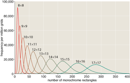
If you generate a bunch of four-colored n-by-n grids at random, the average number of monochromatic rectangles per grid increases quite smoothly with n:
This gradual progression might lead you to suspect that the difficulty of finding or producing an n-by-n grid that is totally devoid of monochrome rectangles would also be a smooth function of n. The truth is quite different.
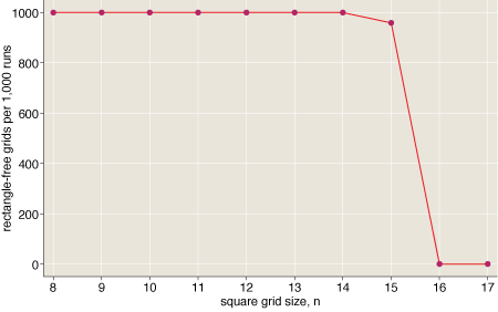
Finding a solution is easy for square grids of any size up to 15 by 15. The task suddenly becomes very hard at size 16 by 16. As for 17 by 17, it’s much harder still–and indeed is not yet known not to be impossible. (Details on the data behind this graph: For each size class from n=8 to n=17 I started with 1,000 randomly four-colored n-by-n grids. Then I applied a simple heuristic search (the first of the algorithms listed below) to each grid, running the program for 1,000 × n2 steps. The graph records the number of times this procedure succeeded–i.e., produced a grid with no monochrome rectangles–at each grid size. Up to n=14, the search never failed; at n=16 and beyond, it never succeeded.)
This kind of sudden transition from easy to hard is a familiar feature in the realm of constraint satisfaction. Well-known intractable problems such as graph coloring and boolean satisfiability have the same structure. That doesn’t bode well for any of the simple-minded computational methods I’ve tried. Here’s a brief catalog of my failures. These are algorithms that I’m pretty sure are never going to pay off.
- Biased random walk. Start with a randomly colored grid. Repeatedly choose a site at random, then try changing its color; accept the move if it reduces the overall number of monochrome rectangles. This is the simplest of all the algorithms. None of the more-elaborate schemes is decisively better.
- Whack-a-mole. Find all the monochrome rectangles in the grid; choose one of them and alter the color of one corner, thereby eliminating the rectangle. In the simplest version of this algorithm, you choose the rectangle and the corner and the new color at random; in more sophisticated versions, you might evaluate the alternatives and take the one that offers the greatest benefit.
- Steepest descent. Examine all possible moves (for the 17-by-17 grid there are 867 of them) and choose one that minimizes the rectangle count.
- Lookahead steepest descent. Examine all possible moves, and then all possible sequels to each such move (for the 17-by-17 grid there are 751,689 two-move sequences); choose a sequence that minimizes the rectangle count. In principle this method could be extended to chains of three or more moves, but the cost soon gets out of hand. (The lookahead technique is the mirror image of backtrack search; it explores the tree of possible moves breadth-first instead of depth-first.)
- Color-balanced search. Allow only moves that maintain the overall balance of colors in the grid. For example, in a 16-by-16 four-colored grid, color balance implies 16 sites in each color. One way to maintain balance is to make moves that swap the colors of two sites. (There is no reason to think that a rectangle-free grid will have exact color balance; on the other hand, a solution for a large grid cannot depart too far from perfect balance. Thus a color-balanced search might be an effective trick for finding a neighborhood where solutions are more common.)
- Row-and-column-balanced search. Allow only moves that maintain the balance of colors within each row and each column of the grid. In a 16-by-16 grid, each row and column should have four sites in each of four colors. A simple way to maintain this detailed color balance is to search for “harlequin rectangles” with the color pattern \(\begin{array}{cc}a & b\\b & a\end{array}\) and permute them to \(\begin{array}{cc}b & a\\a & b\end{array}\).
Most of these techniques are greedy: At each stage the algorithm chooses an action that maximizes some measure of progress. On hard instances, a pure greedy strategy almost always fails; the search gets stuck in some local optimum. Thus it’s usually best to temper the greediness to some extent, occasionally choosing a move other than the one that yields the best immediate return. (The family of methods known as simulated annealing are more elaborate variations on this idea, based on insights from thermal physics.)
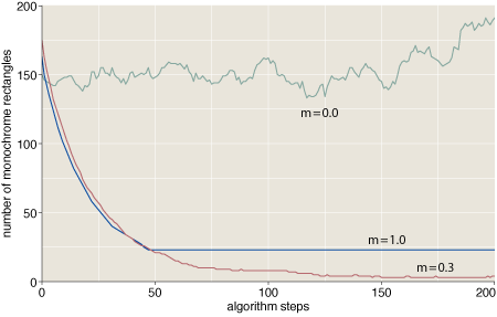
Here we see traces of three runs of the algorithm identified above as steepest descent, with differing values of a greediness parameter m. (The grid size is 15 × 15.) At m=0 (no greediness at all), all moves are equally likely to be chosen, and the algorithm executes a random walk on the space of grid colorings. At m=1 (maximum greediness), the program always chooses the highest-ranked move, which works well until the system stumbles into a state where no move can reduce the rectangle count. A value of m=0.3 seems to be a good compromise. (I’ll say a little more below on the greediness parameter; indeed, I have a question about how best to define and implement it.)
After all this fussing with a dozen variations on local-search algorithms, I’m afraid the outlook for success is not promising. With a little patience and some tuning of parameters, any one of these algorithms can solve grids up to 15 × 15. With a lot more patience and tuning, they’ll eventually yield answers for 16 × 16. But none of the algorithms come even close to cracking the 17 × 17 barrier. Solving that one is going to require a fundamentally new idea. Perhaps someone will find an analytic approach to constructing a solution, rather than blindly searching for one. Or perhaps someone will prove that no solution exists.
On the computational front, I suspect the best hope is a family of algorithms known in various contexts as belief propagation, survey propagation and the cavity method. I’ve been hoping that friends who are expert in these techniques might swoop in and solve the problem for me, but if not I may have to give it a try myself.
In the meantime, here’s the thing about greediness (an apt subject for this time of year?). We want to define a function greedy whose arguments are a vector of alternative moves ranked from best to worst and a number m such that 0 ≤ m ≤ 1. If the greediness parameter m is 0, the function returns a random element of the vector. If m = 1, the returned value is always the first (highest-ranked) move. Otherwise, we must somehow interpolate between these behaviors. One attractive notion is to return the first element of the vector with probability m, the second choice with probability m(1 − m), and so on. Thus for m = 1/2 the series of probabilities would begin 1/2, 1/4, 1/8…. For m = 1/3 the first few values are 1/3, 2/9, 4/27….
This scheme works just fine for a vector of infinite length, but there’s a problem with shorter vectors. Consider what happens with the procedure call greedy(v=[1, 2, 3, 4], m=0.5). We have the following table of probabilities:
     1 --> 1/2
     2 --> 1/4
     3 --> 1/8
     4 --> 1/16
But on adding up those values, we come up 1/16th short of 1. What happens to the missing probability? I took an easy way out, distributing the “extra” probability equally over all the elements of the vector. The code looks something like this:
function greedy(v, m)
  for i=0 to length(v)
     if (i==length(v))
        return v[random(length(v))]
     elseif (random(1.0) < m)
        return v[i]
This procedure seems to give sensible results, but I wonder if there might be a better or more natural definition of greedy probabilities. Also, the running time for my code is logarithmic in the length of the vector (assuming m < 1). Is there a constant-time algorithm that gives the same results? (We don't know the length of the vector in advance, so merely precomputing the table of probabilities is not an option.)