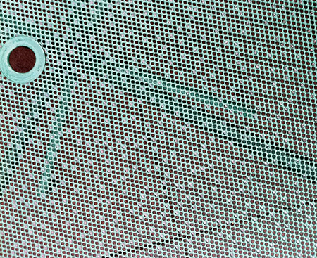
The image above shows the mesh top of a patio table, photographed after a soaking rain. Some of the openings in the mesh retain drops of water. What can we say about the distribution of those drops? Are they sprinkled randomly over the surface? The rainfall process that deposited them certainly seems random enough, but to my eye the pattern of occupied sites in the mesh looks suspiciously even and uniform.
For ease of analysis I have isolated a square piece of the tabletop image (avoiding the central umbrella hole), and extracted the coordinates of all the drops within the square. There are 394 drops, which I plot below as blue dots:
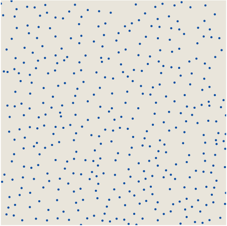
Again: Does this pattern look like the outcome of a random process?
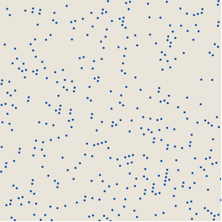
I come to this question in the aftermath of writing an American Scientist column that explores two varieties of simulated randomness: pseudo and quasi. Pseudorandomness needs no introduction here. A pseudorandom algorithm for selecting points in a square tries to ensure that all points have the same probability of being chosen and that all the choices are independent of one another. Here’s an array of 394 pseudorandom dots constrained to lie on a skewed and rotated lattice somewhat like that of the mesh tabletop:
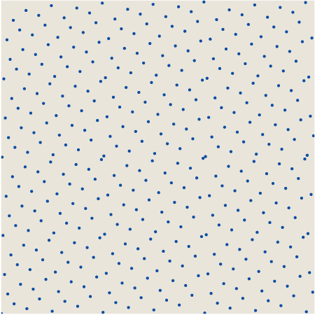
Quasirandomness is a less familiar concept. In selecting quasirandom points the aim is not equiprobability or independence but rather equidistribution: spraying the points as uniformly as possible across the area of the square. Just how to achieve this aim is not obvious. For the 394 quasirandom dots shown below, the x coordinates form a simple arithmetic progression, but the y coordinates are permuted by a digit-twiddling process. (The underlying algorithm was invented in the 1930s by the Dutch mathematician J. G. van der Corput, who worked with one-dimensional sequences, and extended to two dimensions in the 1950s by K. F. Roth. For more details, see my American Scientist column, page 286, or the splendid book by Jiri Matousek.)
Which of these point sets, the pseudo or the quasi, is a better match for the raindrops? Here are the three patterns in miniature, placed side-by-side as an aid to comparison:
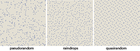
Each of the panels has a distinctive texture. The pseudorandom pattern has both tight clusters and large voids. The quasirandom dots are more evenly spaced (though there are several close pairs of points), but they also form distinctive, small-scale repetitive motifs, most notably a hexagonal structure that repeats with not-quite-crystalline regularity. As for the raindrops, they appear to be spread over the area at almost uniform density (in this respect resembling the quasirandom pattern), but the texture shows hints of swirly rather than latticelike structures (more like the pseudorandom example).
Rather than just eyeballing the patterns, we could try a quantitative approach to describing or classifying them. There are lots of tools for this purpose—radial distribution functions, nearest-neighbor statistics, Fourier methods—but my main motive for bringing up this question in the first place is to play with a new toy that I learned about in the course of reading up on quasirandomness. It is a quantity called discrepancy, which attempts to measure how much a point set departs from a uniform spatial distribution.
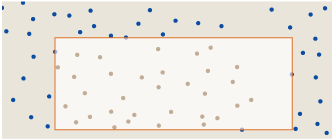
There are lots of variations on the concept of discrepancy, but I’m going to discuss just one measurement scheme. The idea is to superimpose rectangles of various shapes and sizes on the pattern, allowing only rectangles with sides parallel to the x and y axes. Here are three example rectangles drawn on the raindrop pattern:
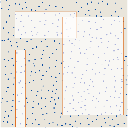
Now count the number of dots enclosed by each rectangle, and compare it with the number of dots that would be enclosed—based on the rectangle’s area—if the distribution of dots were perfectly uniform throughout the square. The absolute value of the difference is the discrepancy D(R) associated with rectangle R:
D(R) = | N · area(R) – #(P ∩ R) |,
where N is the total number of dots and #(P ∩ R) denotes the number of dots P in rectangle R. For example, the rectangle at the upper left covers 10 percent of the area of the square, so its fair share of dots would be 0.1 × 394 = 39.4 dots. The rectangle actually encloses only 37 dots, and so the discrepancy associated with the rectangle is |39.4 — 37| = 2.4. Note that the density of dots in the rectangle could be either higher or lower than the overall average; in either case the absolute-value operation would give a positive discrepancy.
For the pattern as a whole, we can define the global discrepancy D as the worst-case value of this measure, or in other words the maximum discrepancy taken over all possible rectangles drawn in the square. Van der Corput asked whether point sets could be constructed with arbitrarily low discrepancy, so that D would always remain below some fixed bound as N goes to infinity. The answer is No, at least in one and two dimensions; the minimal growth rate is O(log N). Pseudorandom patterns generally have even higher discrepancy, O(√N).
How can you find the rectangle that has maximum discrepancy for a given point set? When I first read the definition of discrepancy, I thought it would be impossible to compute exactly, because there are infinitely many rectangles to be considered. But after thinking about it a while, I realized there are only finitely many candidate rectangles that might possibly maximize the discrepancy. They are the rectangles in which each of the four sides passes through at least one dot. (Exception: Candidate rectangles can also have sides lying on the boundary of the enclosing square.)
Suppose we encounter the following rectangle:
The left, top and bottom sides each pass through a dot, but the right side lies in “empty space.” This configuration cannot be the rectangle of maximum discrepancy. We could push the right edge leftward until it just intersects a dot:
This change in shape reduces the area of the rectangle without altering the number of dots enclosed, and thus increases the density of dots. Alternatively, we could push the edge the other way:
Now we have increased the area, again without changing the count of enclosed dots, and thereby lowered the density. At least one of these actions must increase D(R), compared with the initial configuration. Thus every rectangle with all four sides touching dots or the edges of the square is a local maximum of the discrepancy function; by enumerating all rectangles in this finite set, we can find the global maximum.
There is also the irksome question of whether the rectangle is to be considered “closed” (meaning that points on the boundary are included in the area) or “open” (boundary points are excluded). I’ve sidestepped that problem by tabulating results for both open and closed boundaries. The closed form gives the highest discrepancy for densely populated rectangles, and the open form maximizes discrepancy for sparsely populated rectangles.
By considering only extrema of the discrepancy function, we make the counting problem finite—but not easy! In a square with N dots (all with distinct x and y coordinates), how many rectangles have to be considered? This turns out to be a really sweet little problem, with a simple combinatorial solution. I’m not going to reveal the answer here, but if you don’t feel like working it out for yourself, you could look it up in the OEIS or see a short paper by Benjamin, Quinn, and Wurtz. What I will say is that for N = 394, the number of rectangles is 6,055,174,225—or double that if you count open and closed rectangles separately. For each rectangle, it’s necessary to figure out how many of the 394 points are inside and how many are outside. Pretty big job.
One way to reduce the computational burden is to retreat to a simpler measure of discrepancy. Much of the literature on quasirandom patterns in two or more dimensions uses a quantity called star discrepancy, or D*. The idea is to consider only rectangles “anchored” at the lower left corner of the square (which we can conveniently identify with the origin of the xy plane). In this case the number of rectangles is just N2, or about 150,000 for N = 394.
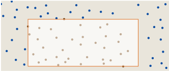
Here is the rectangle that defines the global star discrepancy of the raindrop pattern:
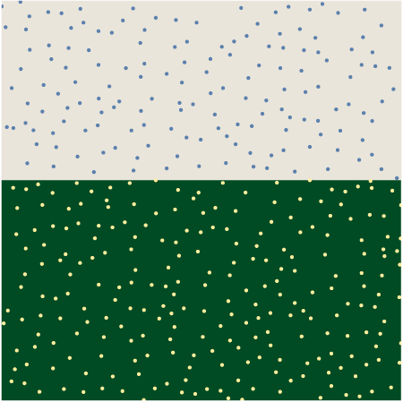
The dark green rectangle at the bottom covers about 55 percent of the square and ought to encompass 216.9 dots, if the distribution were truly uniform. The actual number of dots included (assuming a “closed” rectangle) is 238, for a discrepancy of 21.1. No other rectangle anchored to the corner (0,0) has a greater discrepancy. (Note: Because of limited graphic resolution, the D* rectangle appears to extend horizontally all the way across the unit square; in fact the right edge lies at x = 0.999395.)
What does this result tell us about the nature of the raindrop pattern? Well, for starters, the discrepancy is fairly close to √N (which is 19.8 for N = 394) and not particularly close to log N (which is 6.0 for natural logs). Thus we get no support for the idea that the raindrop pattern might be more quasirandom than pseudorandom. The D* values for the other patterns shown above are in the ranges expected: 25.9 for the pseudorandom and 4.4 for the quasirandom. Contrary to the visual impression, the raindrop distribution seems to have more in common with a pseudorandom point set than a quasirandom one—at least by the D* criterion.
What about calculating the unrestricted discrepancy D—that is, looking at all rectangles rather than just the anchored rectangles of D*? A moment’s thought shows that this exhaustive enumeration of rectangles can’t change the basic conclusion in this case; D can never be less than D*, and so we can’t hope to move from √N toward log N. But I was curious about the computation anyway. Among those six billion rectangles, which one has the greatest discrepancy? Is it possible to answer this question without heroic efforts?
The obvious, straightforward algorithm for D generates all candidate rectangles in turn, measures their area, counts the dots inside, and keeps track of the extreme discrepancies seen along the way. I found that a program implementing this algorithm could determine the exact discrepancy of 100 pseudorandom or quasirandom dots in a few minutes. This outcome might seem to offer some encouragement for pushing on to higher N; however, the running time almost doubles every time N increases by 10, which suggests the computation would take a couple of centuries at N = 394.
I’ve invested a few days’ work in efforts to speed up this calculation. Most of the running time is spent in the routine that counts the dots in each rectangle. Deciding whether a given dot is inside, outside or on the boundary takes eight arithmetic comparisons; thus, at N = 394, there are more than 3,000 comparisons for each of the six billion rectangles. The most effective time-saving device I’ve discovered is to precompute all the comparisons. For each point that can become the lower left corner of a rectangle, I precompute a list of all the pattern dots above and to the right. For each potential upper right corner of a rectangle, I compile a similar list of dots below and to the left. These lists are stored in a hash table indexed by the corner coordinates. Given a rectangle, I can then count the number of interior dots just by taking the set intersection of the two lists.
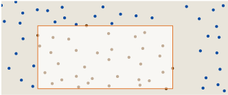
With this trick, the estimated running time for N = 394 came down from two centuries to about two weeks. A big improvement—just enough encouragement to induce me to spend yet another day on further refinements. Replacing the hash table with an N × N array helped a little. And then I figured out a way to ignore all the smallest rectangles, those that cannot possibly be the max-D rectangle because they either contain too few dots or have too small an area. This improvement finally brought the running time down to the overnight range. The illustration below, which shows the rectangle of maximum discrepancy D for the raindrop pattern, took six hours to compute.
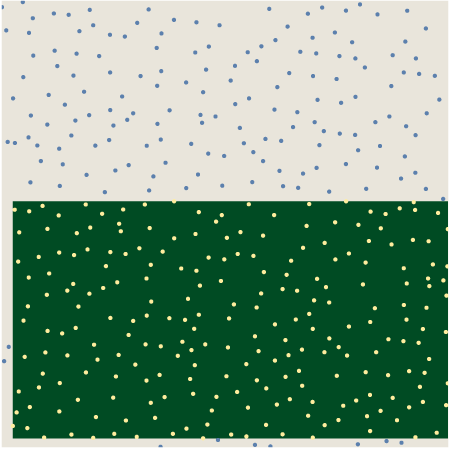
The max-D rectangle is clearly a slight refinement of the D* rectangle for the same point set. The D rectangle “should” contain 204.3 dots but actually has 229, for a discrepancy of D = 24.7. Of course knowing that the exact discrepancy is 24.7 rather than 21.1 tells us nothing more about the nature of the raindrop pattern. As a matter of fact, I feel I know less and less about it as I compute more and more.
When I started this project, I had a pet theory about what might be happening in the tabletop to smooth out the distribution of drops and thereby make the pattern look more quasi- than pseudorandom. To begin with, think of droplets lying on a smooth pane of glass rather than a metal mesh. If two small droplets come close enough to touch, they merge into one larger drop, because that configuration has lower energy associated with surface tension. Perhaps something similar could happen in the mesh. If two adjacent cells of the mesh are both filled with water, and if the metal channel between them is wet, then water could flow freely from one drop to the other. The larger drop will almost surely grow at the expense of the smaller one, and the latter will eventually be annihilated. Thus we would expect a deficit of drops in adjacent cells, compared with a purely random distribution.
This idea still sounds pretty good to me. The only trouble is: It explains a phenomenon that may not exist. I don’t know whether my discrepancy measurements actually reveal anything important about the three patterns, but at the very least the measurements fail to provide evidence that the raindrop distribution is different from the pseudorandom distribution. True, the patterns look different, but how much should we trust our perceptual apparatus in a case like this? If you ask people to draw dots at random, most do a bad job of it, typically making the distribution too smooth and even. Maybe the brain is equally challenged when trying to recognize randomness.
Nevertheless, I suspect there is some mathematical property that will more effectively distinguish between these patterns. If anyone else would like to sink some time into the search, the xy coordinates for the three point sets are in a text file here.
Update 2011-06-24: This is just a brief note to suggest that if you’ve read this far, please go on and read the comments, too. There’s much of value there. I want to thank all those who took the trouble to propose alternative explanations or algorithms, and to point out weaknesses in my analysis. Special thanks to themathsgeek, who within 40 minutes after I first posted the item had come up with a far superior program for computing discrepancies. Also Iain, who pursued my offhand remarks about the perception of random patterns with actual experiments.