
Atlanta. I’m at the Joint Mathematics Meetings, the annual smorgasbord where I never have time to fully digest my helping of algebraic geometry before I move on to a desert of cohomology. Here are a few easily swallowed morsels.
Carey’s Equality. Has everyone but me known all about this for ages and ages?
In a stationary population—where births equal deaths—the number of individuals who have lived a years is the same as the number who still have a years left to live. Here’s a more precise statement from James W. Vaupel of the Max-Planck-Institute for Demographic Research:
If an individual is chosen at random from a stationary population with a positive force of mortality at all ages, then the probability the individual is one who has lived a years equals the probability the individual is one who has that number of years left to live. For example, it is as likely the individual is age 80 as it is the individual has 80 years to live—not 80 years of remaining life expectancy but a remaining lifetime of precisely 80 years.
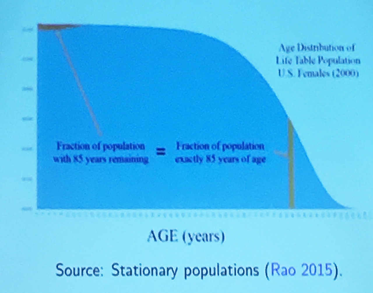
Is this fact obvious, a trivial consequence of symmetry? Or is it deep and mysterious? Apparently it was not clearly recognized until about 10 years ago, by James R. Carey, a biological demographer at UC Davis and UC Berkeley who was studying the age structure of fruitfly populations. The equality was proved in 2009 by Vaupel. A more general statement of the theorem and a more mathematically oriented proof were published in 2014 by Carey and Arni S. R. Srinivasa Rao of Augusta University.
I learned all this from a wide-ranging talk by Rao: “From Fibonacci to Alfred Lotka and beyond: Modeling the dynamics of population and age-structures.”
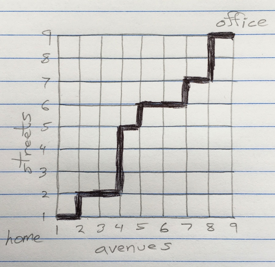
Go with the Green. Every weekday you walk from your home at the corner of 1st Avenue and 1st Street to your office at 9th Avenue and 9th Street. Since your city is laid out with a perfectly rectilinear grid, you have to go eight blocks east and eight blocks north. Assuming you never waste steps by turning south or west, or by straying outside the bounding rectangle, how many routes can you choose from?
It would be quite a chore to count the paths one by one, but combinatorics comes to the rescue. The answer is \(\binom{16}{8}\), the number of ways of choosing eight items (such as eastbound or northbound blocks) from a set with 16 members:
\[\binom{16}{8} = \frac{16!}{(8!)(8!)} = 12{,}870{.}\]
You could walk to work for 50 years without ever taking the same route twice. Which of those 12,870 paths is the shortest? That’s the beauty of the Manhattan metric: They all are. Every such path is exactly 16 blocks long.
But just because the routes are equally long doesn’t mean they are equally fast. Suppose there’s a traffic light at every intersection. Depending on the state of the signal, you can proceed either north or east without interruption, but you’ll have to wait for the light to change if you want to cross the other way. A sensible strategy, it seems, is always to go with the green if you can. Following this rule, you will never have to wait for a light unless you are on the north or the east boundary edge of the square.
The street grid with traffic lights came up in a talk by Ivan Corwin of Columbia University, titled “A Drunk Walk in a Drunk World.” The more conventional term for this subject is “random walks in random environments.” In an ordinary random walk (with a nonrandom environment), the walker chooses a direction at each step according to a fixed probability distribution—the same at all sites and at all times. With a random environment, the probabilities vary both with position and with time. In a brief aside, Corwin offered the street grid with traffic lights as an example of a random environment. If the lights are uncorrelated on the time scale of a pedestrian’s progress through the grid, the favored direction at any intersection is an independent random variable. Then the following question arises: If the walker always takes the green-light direction when that’s possible, which paths are the most heavily traveled?
Corwin’s answer is that the walker will likely follow a stairstep path, never venturing very far from the diagonal drawn between home and office. Thus even though the distance metric says all routes are equal, the walker winds up approximating the Euclidean shortest path.
Corwin gave no proof of his assertion, although he did show the result of a computer simulation. After ruminating on the problem for a while, I think I understand what’s going on. One way of thinking about it is to break the 16-block walk into two eight-block segments, then consider the single vertex that the two segments have in common. Suppose the common point is the central intersection at 5th Avenue and 5th Street. There are 70 ways of getting from home to this point, and for each of those paths there are another 70 ways to continuing on to the office. Thus 4,900 paths pass through the center of the grid. In contrast, only one path goes through the corner of 9th Avenue and 1st Street. The same kind of analysis can be applied recursively to show that the initial eight-block segment of the walk is more likely to pass through 3rd Avenue and 3rd Street than through 5th Avenue and 1st Street.
Another way to look at it is that it’s all about the binomial theorem and Pascal’s triangle. The binomial coefficient \(\binom{n}{m}\) is largest when \(m = n/2\), making the “middle-way” paths the likeliest.
This argument says that always going with the green will give you the fastest route across town (at least in terms of expectation value), and the route you follow is likely to lie near the diagonal. What the argument doesn’t say is that deliberately biasing your choices so that you stay near the diagonal will get you to work sooner; that’s clearly not true.
When I mentioned Corwin’s example to my friends Dan Silver and Susan Williams, Susan immediately pointed out that the model fails to capture some important features of walking in an urban environment. Streets have two sides, and generally two sidewalks. To get from the southwest corner of an intersection to the northeast corner, you need two green lights. I’m not sure whether the conclusions hold up when these complications are taken into account.
I should add that solving this citified problem was not the main point of Corwin’s talk. Instead, he was addressing the problem of a bartender who wants to build a tavern in rough and ever-changing terrain near the rim of the Grand Canyon. The bartender needs to know how close he can come to the edge without endangering inebriated customers who might wander over the cliff.
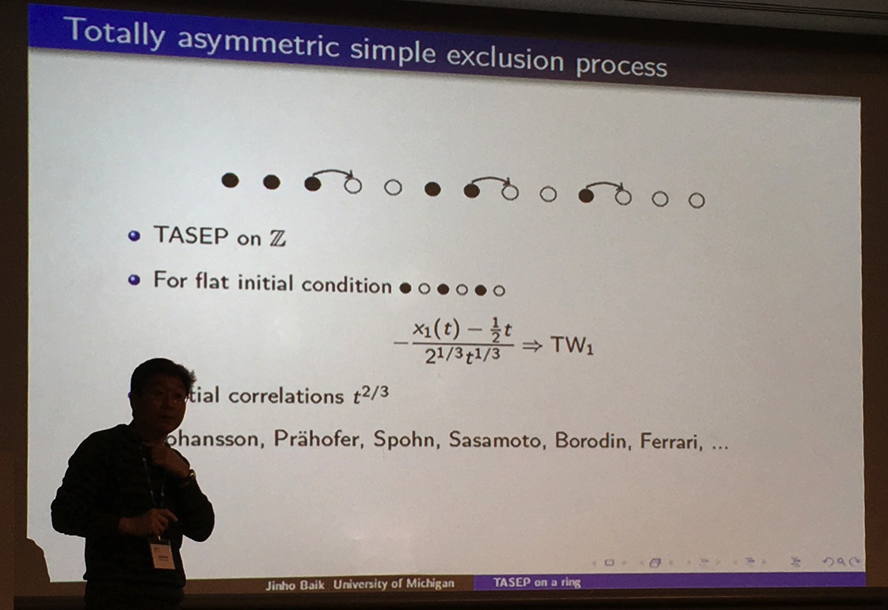
TASEP. I’m a sucker for simple models of complex behavior. This week I learned of a new one—new to me, anyway. Jinho Baik of the University of Michigan talked about TASEP, a “totally asymmetric simple exclusion process” (admittedly not the most vividly descriptive name). Here’s what little I understand of the model so far.
The setting is a one-dimensional lattice, which could be either an infinite line or a closed loop of finite size. Some lattice sites are vacant and some are occupied by a particle. (No site can ever host multiple particles.) At random intervals—random with an exponential distribution—a particle “wakes up” and tries to move one space to the right (on a line) or one space clockwise (on a loop). The move succeeds if the adjacent site is vacant; otherwise the particle goes back to sleep until the next time the exponential alarm clock rings. Given some initial distribution of the particles, how does that distribution evolve over time.
When I see a model like this one, my impulse is to write some code and see what it looks like in action. I haven’t yet done that, but this is my current understanding of what I should expect to see. If you start with the smoothest possible particle distribution (alternating occupied and vacant sites), the particles will tend to clump together. If you start with a maximally clumpy state (one area solidly filled, another empty), the particles will tend to spread out. Baik and his colleagues seek a more precise description of how the density fluctuations evolve over time. And they have found one! Unfortunately, I’m not yet prepared to explain it, even in my hand-waviest way. The best I can do is refer you to the most recent paper by Baik and Zhipeng Liu.
Debunking Guy. If you ever have an opportunity to hear Doron Zeilberger speak, don’t pass it up. At this meeting he gave a spirited and inspiring defense of experimental mathematics, under the title “Debunking Richard Guy’s Law of Small Numbers.” Sitting in the front row was 100-year-old Richard Guy. Neither one of them was in any way daunted by this confrontation. In any case, Doron’s talk was more homage than attack. Later, I had a chance to ask Guy what he thought of it. “His heart is in the right place,” he said.
Guy’s Strong Law of Small Numbers says:
There aren’t enough small numbers to meet the many demands made of them.
As a consequence, if you discover that \(f(n)\) yields the same value as \(g(n)\) for several small values of \(n\), it’s not always safe to assume that \(f(n) = g(n)\) for all \(n\). Euler discovered a cautionary example that’s now well known: The equation \(n^2 + n + 41\) evaluates to a prime for all \(n\) from \(-40\) to \(+39\), but not outside that range.
Zeilberger doesn’t deny the risk of mistaking such accidents for mathematical truths. As a matter of fact, he discusses some of the most dramatic examples: the Pisot numbers, some of which produce coincidences that persist for thousands of terms, and yet ultimately break down. But such pathologies are not a sign that “empirical” mathematics is useless, he says; rather, they suggest the need to refine our proof techniques to distinguish true identities from false coincidences. In the case of the Pisot numbers, he offers just such a mechanism.
A paper by Zeilberger, Neil J. A. Sloane, and Shalosh B. Ekhad (Zeilberger’s computer/collaborator) outlines the main ideas of the JMM talk, though sadly it cannot capture the theatrics.
Soundararajan on Tao on Erdős. Take a sequence of +1s and –1s, and add them up. Can you design the sequence so that the absolute value of the sum is never greater than 1? That’s easy: Just write down the alternating sequence, +1, –1, +1, –1, +1, –1, . . . . But what if, after you’ve selected your sequence, an adversary applies a rule that selects some subset of the entries. Can you still count on keeping the absolute value of the sum below a specified bound? This is a version of the Erdős discrepancy problem, which Paul Erdős first formulated in the 1930s.
The question was finally given a definitive answer in 2015 by Terry Tao of UCLA. In the “Current Events” session of the JMM, Kannan Soundararajan of Stanford gave a lucid account of thre proof. You can read it for yourself, along with three other Current Events talks, by downloading the Bulletin.
Proust’s Powdered-Wig Party. Finally, a personal note. In the closing pages of Marcel Proust’s immense novel A la Recherche du Temps Perdu, the narrator attends a party where he runs into many old friends from Parisian high and not-so-high society. He is annoyed that no one told him the party was a costume ball: All of the guests are wearing white powdered wigs, as if they were gathering at the court of Louis XIV. Then the narrator catches sight of himself in a mirror and realizes that he too is coiffed in white.
At these annual math gatherings I run into people I have known for 30 years or more. For some time I’ve been aware that the members of this cohort, including me, are no longer in the first blush of youth. This year, however, the powdered wigs have seemed particularly conspicuous. Everyone I talk to, it seems, is planning for imminent retirement.
But of course this geriatric impression owes more to selection effects than to the aging of the mathematical population overall. Indeed, the corridors here are full of youngsters attending their first or third or fifth JMM. Which brings us back to Carey’s Equality. If we can safely assume that the population of meeting attendees is stationary, then the proportion of people who have been coming to these affairs for 30 years should be equal to the proportion who will attend 30 more meetings.
Another complication in the Manhattan question that makes a difference in practice is that one can see the lights from some way off and therefore has some idea of when they are next going to change. This means (I think, without analysing it carefully) that if after applying the go-green algorithm one arrives at a point where the direction to the destination is noticeably more horizontal than vertical, which can definitely happen towards the end, and if one has reason to believe that a currently red light that is stopping one going horizontally will soon go green, it may be better to wait for that green in order to avoid reaching the same horizontal level as the destination and then having no choice left about what to do. Or to put it more simply, if you apply the go-green algorithm, you’ll eventually be in the same horizontal or vertical line as your destination, and then you won’t be able to apply it any more. But I would guess (again without doing the analysis so this could be wrong) that if you don’t look at any lights until you get to them and assume some natural distribution on when they will change that’s independent of what has gone before, then going green will be the best thing to do despite this.