
The other day I went over to Danehy Park in Cambridge, which has a fine 400-meter running track. I did four laps at my usual plodding pace. Here is my path, as recorded by an iPhone app called Runmeter:
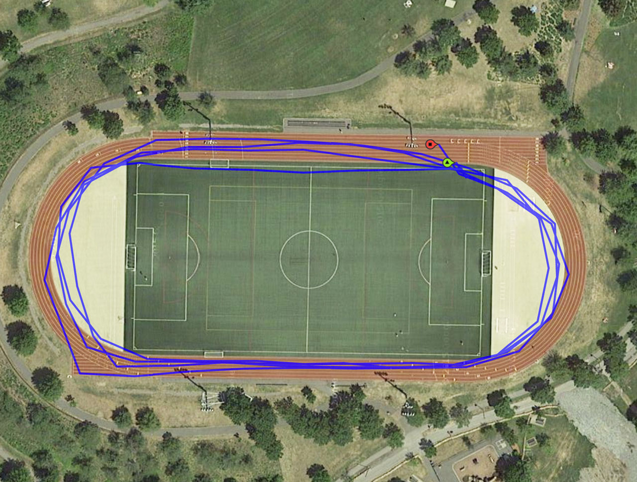
No, I wasn’t drunk. The blue trace shows me lurching all over the track, straying onto the soccer field, and taking scandalous shortcuts in the turns—but none of that happened, I promise. During the entire run my feet never left the innermost lane of the oval. All of my apparent detours and diversions result from GPS measurement errors or from approximations made in reconstructing the path from a finite set of measured positions.
At the end of the run, the app tells me how far I’ve gone, and how fast. Can I trust those numbers? Looking at the map, the prospects for getting accurate summary statistics seem pretty dim, but you never know. Maybe, somehow, the errors balance out.
Consider the one-dimensional case, with a runner moving steadily to the right along the \(x\) axis. A GPS system records a series of measured positions \(x_0, x_1, \ldots, x_n\) with each \(x_i\) displaced from its true value by a random amount no greater than \(\pm\epsilon\). When we calculate total distance from the successive positions, most of the error terms cancel. If \(x_i\) is shifted to the right, it is farther from \(x_{i-1}\) but closer to \(x_{i+1}\). For the run as a whole, the worst-case error is just \(\pm 2 \epsilon\)—the same as if we had recorded only the endpoints of the trajectory. As the length of the run increases, the percentage error goes to zero.
In two dimensions the situation is more complicated, but one might still hope for a compensating mechanism whereby some errors would lengthen the path and others shorten it, and everything would come out nearly even in the end. Until a few days ago I might have clung to that hope. Then I read a paper by Peter Ranacher of the University of Salzburg and four colleagues. (Take your choice of the journal version, which is open access, or the arXiv preprint. Hat tip to Douglas McCormick in IEEE Spectrum, where I learned about the story.)
Ranacher’s conclusion is slightly dispiriting for the runner. On a two-dimensional surface, GPS position errors introduce a systematic bias, tending to exaggerate the length of a trajectory. Thus I probably don’t run as far or as fast as I had thought. But to make up for that disappointment, I have learned something new and unexpected about the nature of measurement in the presence of uncertainty, and along the way I’ve had a bit of mathematical adventure.
The Runmeter app works by querying the phone’s GPS receiver every few seconds and recording the reported longitude and latitude. Then it constructs a path by drawing straight line segments connecting successive points.
Two kinds of error can creep into the GPS trajectory. Measurement errors arise when the reported position differs from the true position. Interpolation errors come from the connect-the-dots procedure, which can miss wiggles in the path between sampling points. Ranacher et al. consider only the inaccuracies of measurement, on the grounds that interpolation errors can be reduced by more frequent sampling or a more sophisticated curve-fitting method (e.g., cubic splines rather than line segments). Interpolation error is eliminated altogether if the runner’s path is a straight line.
Suppose a runner on the \(x, y\) plane shuttles back and forth repeatedly between the points \(p = (0, 0)\) and \(q = (d, 0)\). In other words, the end points of the path lie \(d\) units apart along the \(x\) axis. After \(n\) trips, the true distance covered is clearly \(nd\). A GPS device records the runner’s position at the start and end of each segment, but introduces errors in both the \(x\) and \(y\) coordinates. Call the perturbed positions \(\hat{p}\) and \(\hat{q}\), and the Euclidean distance between them \(\hat{d}\). Ranacher and his colleagues show that for large \(n\) the total GPS distance \(n \hat{d}\) is strictly greater than \(nd\) unless all the measurement errors are perfectly correlated.
I wanted to see for myself how measured distance grows as a function of GPS error, so I wrote a simple Monte Carlo program. The Ranacher proof makes no assumptions about the statistical distribution of the errors, but in a computer simulation it’s necessary to be more concrete. I chose a model where the GPS positions are drawn uniformly at random from square boxes of edge length \(2 \epsilon\) centered on the points \(p\) and \(q\).
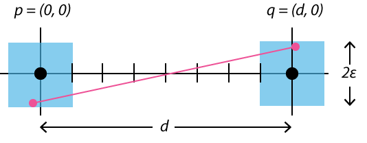
In the sketch above, the black dots, separated by distance \(d\), represent the true endpoints of the runner’s path. The red dots are two GPS coordinates \(\hat{p}\) and \(\hat{q}\), and the red line gives the measured distance between them. We want to know the expected length of the red line averaged over all possible \(\hat{p}\) and \(\hat{q}\).
Getting the answer is quite easy if you’ll accept a numerical approximation based on a finite random sample. Write a few lines of code, pick some reasonable values for \(d\) and \(\epsilon\), crank up the random number generator, and run off 10 million iterations. Some results:
| \(\epsilon\) | \(d\) | \(\hat{d}\) |
|---|---|---|
| 0.0 | 1.0 | 1.0000 |
| 0.1 | 1.0 | 1.0034 |
| 0.2 | 1.0 | 1.0135 |
| 0.3 | 1.0 | 1.0306 |
| 0.4 | 1.0 | 1.0554 |
| 0.5 | 1.0 | 1.0882 |
For each value of \(\epsilon\) the program generated \(10^7\) \((\hat{p}, \hat{q})\) pairs, calculated the Euclidean distance \(\hat{d}\) between them, and finally took the average \(\langle \hat{d} \rangle\) of all the distances. It’s clear that \(\langle \hat{d} \rangle > d\) when \(\epsilon > 0\). Not so clear is where these particular numbers come from. Can we understand how \(\hat{d}\) is determined by \(d\) and \(\epsilon\)?
For a little while, I thought I had a simple explanation. I reasoned as follows: We already know from the one-dimensional case that the \(x\) component of the measured distance has an expected value of \(d\). The \(y\) component, orthogonal to the direction of motion, is the difference between two randomly chosen points on a line of length \(2 \epsilon\); a symmetry argument gives this length an expected value of \(2 \epsilon / 3\). Hence the expected value of the measured distance is:
\[\hat{d} = \sqrt{d^2 + \left(\frac{2 \epsilon}{3}\right)^2}\, .\]
Ta-dah!
Then I tried plugging some numbers into that formula. With \(d = 1\) and \(\epsilon = 0.3\) I got a distance of 1.0198. The discrepancy between this value and the numerical result 1.0306 is much too large to dismiss.
What was my blunder? Repeat after me: The average of the squares is not the same as the square of the average. I was calculating the squared distance as \({ \langle x \rangle}^2 + {\langle y \rangle}^2 \) when what I should have been doing is \(\langle {x^2 + y^2}\rangle\). We need to average over all possible distances between a point in one square and a point in the other, not over all \(x\) and \(y\) components of those distances. Trouble is, I don’t know how to calculate the correct distance.
I thought I’d try to find an easier problem. Suppose the runner stops to tie a shoelace, so that the true distance \(d\) drops to zero; thus any movement detected is a result of GPS errors. As long as the runner remains stopped, the two error boxes exactly overlap, and so the problem reduces to finding the average distance between two randomly selected points in the unit square. Surely that’s not too hard! The answer ought to be some simple and tidy expression—don’t you think?
In fact the problem is not at all easy, and the answer is anything but tidy. We need to evaluate a terrifying quadruple integral:
\[\iiiint_0^1 \sqrt{(x_q - x_p)^2 + (y_q - y_p)^2} \, dx_p \, dx_q \, dy_p \, dy_q\, .\]
Lucky for me, I live in the age of MathOverflow and StackExchange, where powerful wizards have already done my homework for me.
\[\frac{2+\sqrt{2}+5\log(1+\sqrt{2})}{15} \approx 0.52140543316\]
Nothing to it, eh?
The corresponding expression for nonzero \(d\) is doubtless even more of a monstrosity, but I’ve made no attempt to derive it. I am left with nothing but the Monte Carlo results. (For what it’s worth, the simulations do agree on the value \(\hat{d} = 0.5214\) for \(d = 0\)).
I tried applying the Monte Carlo program to my 1,600-meter run. In the Runmeter data my position is sampled 100 times, or every six seconds on average, which means that \(d\) (the true average distance between samples) should be about 16 meters. Estimating \(\epsilon\) is not as easy. In the map above there’s one point on the blue path that’s displaced by at least 10 meters, but if we ignore that outlier most of the other points are probably within about 3 meters of the correct lane. Plugging in \(d = 16\) and \(\epsilon = 3\) yields about 1,620 meters as the expected measured distance.
What does the Runmeter app have to say? It reports a total distance of 1,599.5 meters, which is, I’m inclined to say, way too good to be true. Part of the explanation is that the measurement errors are not uniform random variables; there are strong correlations in both space and time. Also, measurement errors and interpolation errors surely have canceled out to some extent. (It’s even possible that the developers of the app have chosen the sampling interval to optimize the balance between the two error types.) Still, I have to say that I am quite surprised by this uncanny accuracy. I’ll have to run some more laps to see if the performance is repeatable.
Another thought: People have been measuring distances for millennia. How is it that no one noticed the asymmetric impact of measurement errors before the GPS era? Wouldn’t land surveyors have figured it out? Or navigators? Distinguished mathematicians, including Gauss and Legendre, took an interest in the statistical analysis of errors in surveying and geodesy. They even did field work. Apparently, though, they never stumbled on the curious fact that position errors orthogonal to the direction of measurement lead to a systematic bias toward greater lengths.
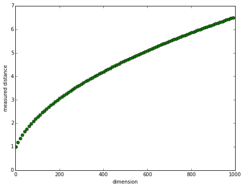
There’s yet another realm in which such biases may have important consequences: measurement in high-dimensional spaces. Inaccuracies that cause a statistical bias of 2 percent in two-dimensional space give rise to a 19 percent overestimate in 10-dimensional space. The reason is that errors along all the axes orthogonal to the direction of measurement contribute to the Euclidean distance. By the time you get to 1,000 spatial dimensions, the measured distance is more than six times the true distance.
Even for creatures like us who live their lives stuck in three-space, this observation might be more than just a mathematical curiosity. Lots of algorithms in machine learning, for example, measure distances between vectors in high-dimensional spaces. Some of those vectors may be closer than they appear.
Is it possible that Runkeeper detected — through a lookup table of known tracks, or just by analyzing the shape of your trace — that you were running around a 400 meter track and adjusted its measured total accordingly?
At my local high school track, slow pokes are asked to use the outer lanes so that folks doing a serious workout (intervals, etc.) can use the inside lanes. This correction would make us slow pokes even more discouraged at our slow paces!
Ah, yes, like the compiler that recognizes the LINPACK benchmarks and optimizes away the whole computation. Seems rather a lot of trouble, don’t you think?
Was that only GPS or GPS with assist of some service. My phone (Galaxy S5) always done very well with drawing paths. I’m using Nike+ Running application w/ all GPS services open (GPS & Wi-Fi & Mobile Network together).
The app’s decumentation mentions only GPS, and it refuses to start recording if it can’t get a GPS fix. In any case, the track I was running on is built atop an old sanitary landfill and is a few hundred meters from the nearest buildings; wifi reception can’t be very good up there.
What matters isn’t the expected distance, but rather the variance. If you know that the expected distance is 1.08, then the software can just divide everything by 1.08 to fix this systematic error. I don’t know how sophisticated your particular software is, but I wouldn’t expect the authors to be completely mathematically naive.
If the app were simply trying to give a best estimate of total distance, your strategy would be appealing. But the app is doing more than that: It plots position and speed at frequent intervals. All the waypoints along the trajectory somehow have to be reconciled with the total speed and distance. I suppose you could apply the adjustment to each segment of the path, but I don’t believe that’s being done.
The app dumps the position data in a file format called KML (an XML variant). The file includes the full list of lat/lon pairs (in decimal degrees, e.g., 42.3891314, -71.1362197) and the distances between successive points calculated to a precision of one-tenth meter. I have checked that the distances listed in the file have not been adjusted. I calculated the great-circle distances between successive points, using the haversine algorithm; the results agree with the distances in the KML file to within the roundoff error.
Very interesting! Wouldn’t the space for \( \hat{p} \) be a circle of radius \( \epsilon \), rather than a square of edge \( 2\epsilon \) ?
Also, for your experiment you could try to gather the raw GPS location data using a GPS app, rather than rely on an app such as Runkeeper which may have some corrective algorithm in place. “GPS Test, Coordinates, Logger - FREE” was the first to come up on a Google search for such Android apps.
Thanks for the article, was a great read!
An error circle does indeed seem more plausible than an error square. In my first calculations I actually used a two-dimensional normal distribution, which seemed even more likely than a uniform circular one. But when I started trying to work out a closed-form expression for the distance between two random points, I wanted the simplest case possible, and having independent, uniformly distributed x and y variables seemed like the best bet.
I agree that using a black-box app like Runmeter is not the best approach. The Ranacher paper includes some experiments done with better technology.
Faith in GPS is fodder for jokes. Radio waves are subject to all kinds of changes as they pass thru the atmosphere from space. Many of these changes are due to weather, therefore not repeatable. GPS is good enough to get a missile warhead close enough to its target, most of the time. That’s the design constraint. Math and digital gizmos are not the same as the real world, and never will be. Get used to it. Reality, what a concept.
I found there is an easy 20-50 meter discrepancy when dealing with GPS during my development projects.
It is also very much weather dependent.
perhaps because you notice when you perform a “path integral”. before gps only distances between reference landmarks were measured since the measurement process was extremely cumbersome. only recently could one consider to measure continously in an easy way.
I always notice the same when recording tracks with my Garmin Dakota 20.
Sometimes, when you have several paths relatively close to each other, but on different altitudes, it is quite difficult to see which one I followed.
When walking in woods, the effect gets even worse.
It disappointed me quite a lot, the first times I noticed this. Now, I just clean up these tracks while I can still remember what the correct path was. But I still feel this is not worthy the current state of technology.