
I went to a magic show the other day. Nick Trefethen was giving a demo of Chebfun, a Matlab extension package he is building in collaboration with his Oxford students and colleagues. In the course of the talk, several mathematical rabbits were pulled out of numerical hats.
The key idea in Chebfun is to represent any function of a real variable by a polynomial approximation.
  >> f = chebfun('sin(x) + sin(x.^2)', [0 10]);
  >> plot(f)
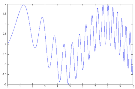
That wiggly line looks like a graph of y = sin(x) + sin(x2), but that’s an illusion. What is being plotted here is a certain polynomial of degree 118 that happens to approximate sin(x) + sin(x2) with high precision.
As I understand it, the chebfun construction algorithm works something like this. First you select N+1 points in the interval where the function is defined, and construct the unique polynomial of degree N that passes through all the points. If the error of this approximation is below a threshold, you’ve found your chebfun. Otherwise, choose a larger sample of points and try again.
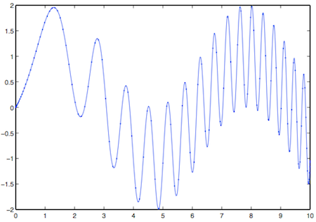
The sample points are not evenly spaced across the interval. They are Chebyshev points, whose distribution varies as a cosine function, denser at the extremes and sparser in the middle. In this case, the process converged with 119 Chebyshev points:
In one respect the example above is an easy one: The function is quite smooth. Here’s something more challenging:
  >> hat = 1-abs(x-5)/5;
  >> h = max(f, hat);
  >> plot(h)
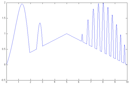
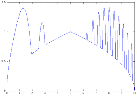
This is where we pull the rabbit out of the hat—or at least several pairs of rabbit ears. To deal with the discontinuities sharp corners in this curve, the Chebfun system assembles 25 polynomial segments, each defined on a different interval. Some are linear, some of higher degree. But the entire structure is still treated as a single function, which can be operated on by other functions. For example, sum(h) calculates the integral over [0, 10], returning the result 8.598303617326401. And here’s the square root of those rabbit ears:
These are neat tricks, but why would one want to work with polynomial approximations to a function, rather than with the function itself? I’m too new to all this to answer that question with confidence, so I’ll quote the Chebfun Guide:
The aim of Chebfun is to “feel symbolic but run at the speed of numerics”. More precisely our vision is to achieve for functions what floating-point arithmetic achieves for numbers: rapid computation in which each successive operation is carried out exactly apart from a rounding error that is very small in relative terms.
For those who want to know more, I offer a few pointers:
The first published paper on Chebfun:
Battles, Zachary, and Lloyd N. Trefethen. 2004. An extension of MATLAB to continuous functions and operators. SIAM Journal on Scientific Computing 25:1743–1770. (PDF)
Trefethen’s argument favoring floating-point arithmetic over symbolic computation or exact rational arithmetic:
Trefethen, Lloyd N. 2007. Computing numerically with functions instead of numbers. Mathematics in Computer Science 1:9–19. (PDF)
A provocative account of why polynomial approximation is not as wonky as you may think:
Trefethen, Lloyd N. 2011. Six myths of polynomial interpolation and quadrature. Mathematics Today. (PDF)
Finally, Trefethen has a forthcoming book on Chebfun and related matters (which I have only just begun to read):
Trefethen, Lloyd N. To appear. Approximation Theory and Approximation Practice. (PDF)
Chebfun runs inside Matlab, the numerical computing environment from Mathworks. Chebfun itself has recently become open-source software (under a BSD license), but Matlab is proprietary. As far as I can tell, Chebfun does not not (yet?) run under Octave, the open-source alternative to Matlab.
Just a brief observation. You mentioned it’s necessary to deal with the discontinuities in max(f, hat), but this function is actually continuous. I think you meant to say it’s not differentiable.
@Damon McDougall: Thanks. Of course you’re quite right. But I now discover a gap in my mathematical vocabulary. If those points are not to be called discontinuities, what do we call them? When we speak of the curve as a whole, we have a nice collection of adjectives for various properties—continuous, smooth, differentiable (and their negations). But how do we describe a point that makes a curve nondifferentiable? Is there some term in common use that I’ve forgotten or never learned?
When I was an undergrad we would call points at which the function is continuous but the first derivative is not a “kink”. We might have gotten this from Spivak or Rudin’s book. I doubt this is standard nomenclature, though.
Sorry I meant:
points at which the function is continuous but the first derivative does not exist.
Hi:
I am also one of those wanting to try Chebfun in a non-MatLab environment/software.
Python is a good bet
as its scipy/numpy have a lot of built in routines on Chebyshev polynomials but they are still not so user friendly.
Recently I came across a laudable effort by a couple of Cornell
grad students Alex and Alemi who have hosted the 0.1th version of their Pychebfun package on GitHub. This is downloadable as a zipped folder
and the pychebfun.py program therein brings the full power of scipy/numpy into any user’s hands.
The command at the top is executed in python27 as:
from __future__ import division
from scipy import *
from pylab import *
from pychebfun import *
f = chebfun(‘sin(x) + sin(x**2)’, [0 10]);
f.plot() # –> draws same figure !
print f.quad()
outputs ” N = 126 ; domain: (0, 10) ;f.quad(): 2.42274242900607195″
This value is almost the same as in Chebfun webpage!
Similarly differentiation, integration, rootfinding etc can also be done easily.
All these are worth a try.
Mr Webmaster: Please rectify a fault of this page whereby after submission sender’s email and name are not deleted and reset!
Thank you
Mr Webmaster :
Why don’t you add a “reset” button at least to clear this window?
Thank you