Orderly Randomness
Quasirandom Numbers and Quasi–Monte Carlo
Brian Hayes
Harvard Institute for Applied Computational Science, 2015-02-06
Slides at: bit-player.org/extras/quasi
Part 1
Integration by Darts

Random Sampling
Darts:
Hits:
Area:
True area: 0.4178
Lattice Sampling
Darts:
Hits:
Area:
True area: 0.4178
Quasirandom Sampling
Darts:
Hits:
Area:
True area: 0.4178
Part 2
Varieties of Randomness
| • eurandom | (eu = good, true) |
| • pseudorandom | (pseudo = false, fake) |
| • quasirandom | (quasi = as if, seemingly) |
| • nonrandom | (non = not) |
Eurandom Numbers
- Unpredictable. (Also unrepeatable.)
- Uncorrelated, or independent.
- Unbiased, or uniformly distributed.
Eurandom Numbers
- Adversarial contexts: cryptography, gambling, proof.
- Need a source of entropy.
- A curious link between mathematics and physics, between the world of bits and the world of atoms.
Eurandom Numbers
- The gold standard, yet famously unreliable.
- Weldon and Tebb: after many years of rolling dice for science, Karl Pearson found an excess of fives and sixes.
- Almost always, the raw bits need to be “whitened.”
What could possibly go wrong?
A prime number for a cryptographic key, produced by the random number generator on a certain “smart card”:
					10055855947456947824680518748654384595609524365
					44429503329267108279132302255516023260140572362
					51775707675238936398645381403154121089599274598
					25236754563833
The same number written in binary:
					11000000000000000000000000000000000000000000000
					00000000000000000000000000000000000000000000000
					00000000000000000000000000000000000000000000000
					00000000000000000000000000000000000000000000000
					00000000000000000000000000000000000000000000000
					00000000000000000000000000000000000000000000000
					00000000000000000000000000000000000000000000000
					00000000000000000000000000000000000000000000000
					00000000000000000000000000000000000000000000000
					00000000000000000000000000000000000000000000000
					000000000000000000000000000000001011111001
Pseudorandom Numbers
- Unpredictable. (Also unrepeatable.)
- Uncorrelated, or independent.
- Unbiased, or uniformly distributed.
Pseudorandom Numbers
Any one who considers arithmetical methods of producing random digits is, of course, in a state of sin.—von Neumann (1951)
Subtle is the Lord..., but he’s not out to get us.—Einstein (1921)
Pseudorandom Numbers
- Commonly generated by a linear recurrence, e.g.: \(x_k = a x_{k-1} + b \pmod{m}\).
- Not really uncorrelated: Finite cycle length, at most \(m\).
- Not really unbiased: Runs of 0s underrepresented.
Pseudorandomness: The Full Monte
\(x_k = 41 x_{k-1} + 1 \pmod{256},\quad x_0 = 3\)
Quasirandom Numbers
- Unpredictable. (Also unrepeatable.)
- Uncorrelated, or independent.
- Unbiased, or uniformly distributed.
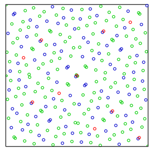
Quasirandom Patterns
Quasirandom Numbers
- We’re in the realm of deterministic machines.
- They don’t pretend to be random.
- They don’t even look random.
What Is Randomness?
Philosophical musings
Part 3
A Slight Discrepancy
Counting points and measuring volume in axis-aligned rectangles

\[D(a,b) = \left\lvert\frac{\mathrm{count}[a,b)^2}{\mathrm{count}[0,1)^2} - \frac{\mathrm{vol}[a,b)^2}{\mathrm{vol}[0,1)^2}\right\rvert\]
Counting points and measuring volume in axis-aligned rectangles
\[D(a,b) = \left \lvert \mathrm{count}[a,b)^2 - \mathrm{count}[0,1)^2 \frac{\mathrm{vol}[a,b)^2}{\mathrm{vol}[0,1)^2}\right\rvert\]
Worst-case measure: \(\max\) over all axis-aligned rectangles \([a,b)^2\)
\[D = \max_{[a,b)^2 \in [0,1)^2} \left\lvert\frac{\mathrm{count}[a,b)^2}{\mathrm{count}[0,1)^2} - \frac{\mathrm{vol}[a,b)^2}{\mathrm{vol}[0,1)^2}\right\rvert\]
Star discrepancy: axis-aligned anchored rectangles

\[D* = \max_{[0,b)^2 \in [0,1)^2} \left\lvert\frac{\mathrm{count}[0,b)^2}{\mathrm{count}[0,1)^2} - \frac{\mathrm{vol}[0,b)^2}{\mathrm{vol}[0,1)^2}\right\rvert\]
Part 4
Quasi History
Mathematical Origins
- Ergodic theory: Well-stirred systems.
- Can we fill the unit interval uniformly?
- Simple arithmetic progression seems to be the answer.
- But how do we add points one at a time while preserving uniformity?
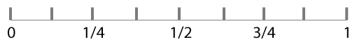
Covering the Interval [0, 1)
- Hermann Weyl 100 years ago: the sequence \(\alpha, 2\alpha, 3\alpha,\dots,n\alpha \pmod{1}\) is equidistributed if \(\alpha\) is any irrational number.
- Proved by an argument about Riemann integrals that leads directly to the idea of Monte Carlo integration.
- Irrationality is necessary; without it, only a finite set of fractions.
- Irrationality is inconvenient for finite computing machines.
Covering the Interval [0, 1)
- Johannes van der Corput, 1930s: Asked if any sequence could have discrepancy bounded by a constant for all N.
- In other words, if the discrepancy is given by some function \(f(N)/N\), can \(f(N)\) remain below some constant \(C\) as \(N\) goes to infinity?
- The answer is no. Proved in the 1940s by Tatyana Pavlovna van Aardenne-Ehrenfest.
- Stronger bounds by K. F. Roth in the 1950s, and others.
- Extensions to point sets in two or more dimensions.
A First Attempt
at Quasi-MC
- R. D. Richtmyer, Los Alamos, 1951.
- Problem of neutron diffusion (same as first MC studies).
- A Weyl sequence: \(n \alpha \pmod 1 \) for irrational \(\alpha\).
- Outcome: No better than ordinary Monte Carlo.
- But he published the negative result! (This is to be encouraged: You can claim priority even for your failures.)
Part 5
Making Quasirandom Numbers
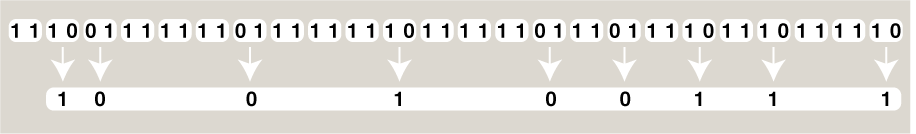
Van der Corput Procedure
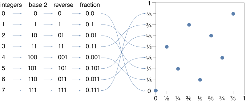
Quasirandomness Generators
- Van der Corput algorithm is a bizarre mashup of operations on numbers and operation on numerals—the representation of numbers.
- Other quasirandom generators are just as strange.
- Maybe this sort of bit-twiddling is where the “randomness” comes from in quasirandom sequences.
I. M. Sobol Quasipattern
Part 6
Convergence Rates
Convergence Rates
- How many points do you have to sample to achieve a given accuracy?
- For pseudorandom Monte Carlo, the expected sampling error is proportional to \(\sqrt{N}/N\).
- This bound follows from the law of large numbers or the central limit theorem.
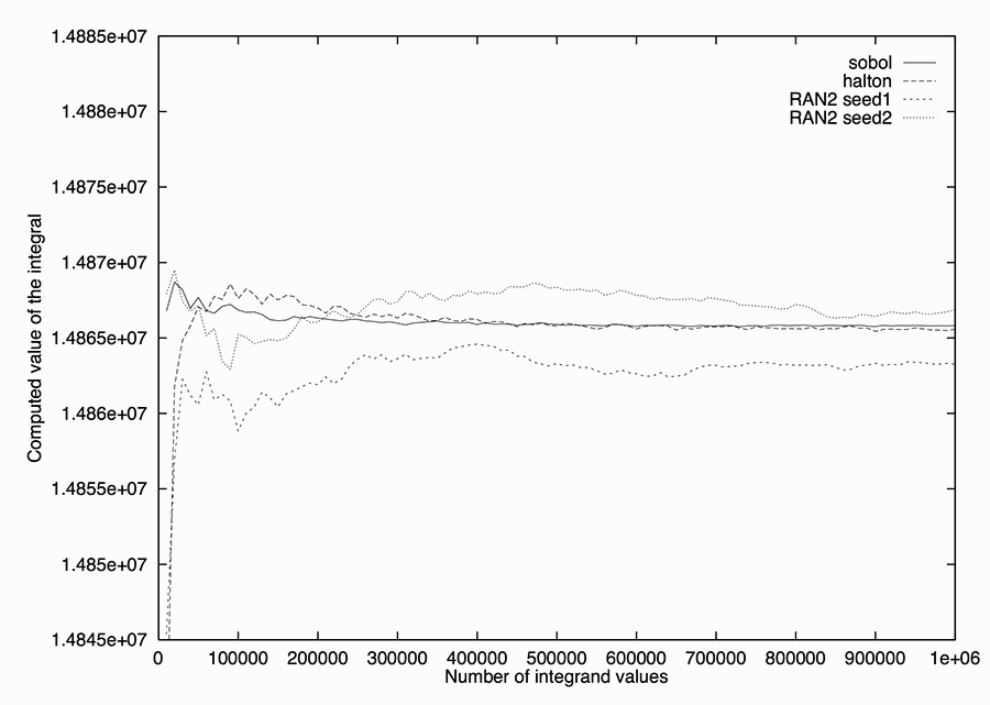
Convergence Rates
- In quasi-Monte Carlo, the corresponding expected error goes as \((\log N)^{d}/N\), where \(d\) is the spatial dimension.
- Trading \(\log N\) for \(\sqrt{N}\) is potentially a huge improvement: the square root of 1,000,000 is 1,000, but \(\log_{2}\) 1,000,000 is only 20.
- But there’s that pesky exponent \(d\). For any fixed \(d\), \(\sqrt{N}/N\) will eventually exceed \((\log N)^{d}/N\), but it may take a very large value of \(N\) to reach the crossover.
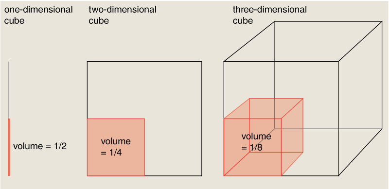
The Curse of Dimensionality
- In high dimensions, all the volume is in the corners.
- Measuring that volume, effort grows as \(2^d\).
Another Problem: Error Estimates
- Randomness in conventional MC yields an intrinsic error estimate: Just measure the variance of multiple trials.
- Deterministic methods (quasi or lattice) have no concept of variance.
The Twilight of Quasi-MC
The situation from the 1950s into the 1990s:
- Quasi-Monte Carlo has a theoretical advantage in low dimensions.
- But most low-dimensional problems are easy for any numeric integration scheme.
- For pseudorandom MC, the \(\sqrt{N}\) convergence rate is less than wonderful, but it does have the virtue of being independent of dimension.
- As a result, quasi-MC was largely set aside by practitioners, although mathematical work continued.
Part 7
A New Dawn for Quasi-MC
Financial Engineering
- Collateralized mortgage obligation (CMO): One of the clever inventions that brought us the great recession of 2008.
- Gathers thousands of mortgage loans into a single, marketable security.
- Whether you’re buying or selling, you need a way to assign a price to a specific CMO.
Pricing a CMO
- Isn’t this a straightforward problem of calculating net present value?
- A 30-year mortgage represents a stream of 360 monthly payments; you apply a discount rate to determine how much you ought to pay now for the promise of a dollar 30 years hence.
- But most mortgages do not survive for a full 360 monthly payments. When a house is sold or refinanced, the balance is paid in advance. There’s also the possibility of default.
Monte Carlo on Wall Street
- Formulate the problem as an integral in a space of 360 dimensions.
- For evaluating such integrals Monte Carlo methods are favored not because they work well but because nothing else works at all.
- The use of such techniques, borrowed from physics or computer science, became part of the great “quant” revolution in finance in subsequent years.
Quasi-Monte Carlo on Wall Street
- In 1992 Goldman Sachs, the investment bank, approached Joseph Traub’s group at Columbia seeking advice on methods for evaluating CMOs.
- Traub and several graduate students, including Spassimir Paskov, decided to try quasi-Monte Carlo, ignoring the received wisdom.
- It worked. Convergence was faster by a factor between 2 and 5.
The Aftermath
- Paskov earned his degree and went to work for a Swiss bank.
- Traub, Paskov, and another colleague received a patent related to the work.
- Use of quasi-MC spread rapidly through the world of investment banking.
- Twelve years later, the economy tanked. (Causation?)
- Meanwhile, the small community of quasi-fanatics went to work figuring out what it all means.
Part 8
Quasi Miracles?
Laws of Nature Still Enforced
- The earlier results on convergence rates and accuracy were not wrong.
- The curse of dimensionality has not been lifted.
- Fully evaluating a 360-dimensional integral requires \(\approx 2^{360}\) samples, not \(10^{6}\).
- \(\therefore\) either the quasi-MC technique is more powerful than we knew, or the problem is easier than it looks.
Effective Dimensions?
- The Paskov-Traub result provoked a spate of quasi reassessments (e.g., [Caflisch 1998], [Owen 2002], [Sloan 2005].
- The verdict: The 360-dimensional integral doesn’t really have 360 “effective” dimensions.
- ANOVA approach: If almost all the variance lies in a few dimensions, the rest can be truncated.
- Analogous to compressed-sensing.
Open Questions
- How do we recognize that a problem has effective dimensionality lower than its formal dimensionality?
- How common are such problems?
- Will quasirandom methods work for other kinds of Monte Carlo studies (e.g., random walks, percolation, statistical mechanics, optimization)?
Thanks!
Bibliography (PDF)
brian@bit-player.org
Start Over