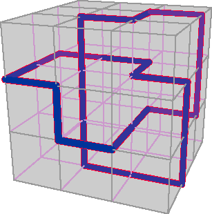
Figure 1. Smallest knot on the cubic lattice is a trefoil 24 units long.
Life would be so much simpler if only we lived in Z3 instead of R3. Here at home in R3, every point in space has coordinates drawn from the set of real numbers, R (a set that encompasses the integers, the rationals and the irrationals). Nature seems content with this arrangement, but ever since the time of Zeno, people trying to understand the structure of the physical world have puzzled over the way points get squished together at infinite density on the real-number line. This numerical overcrowding is particularly troublesome when you try to simulate nature with a digital computer. Computer programs have a hard time with the continuum of real numbers; they trip over concepts such as the identity 0.999... = 1.0.
Z3 is a more computer-friendly place. Here all points have integer coordinates (drawn from the set of positive and negative whole numbers, Z). You can think of Z3 as a cubic lattice, like a crystal of salt. The nodes of the lattice--the spots occupied by atoms in the crystal--are the only points that exist. To move through the lattice, you jump from node to node, without ever passing through intermediate positions. Where R3 is a jungle whose dense undergrowth has to be hacked away, Z3 is a tidy urban space, where everything is discrete and countable, arranged in rows and columns.
A lattice is an especially good place for doing computational science, because the discrete space maps so readily onto the discrete structures of the computer. In models based on cellular automata, for example, each node of the lattice is imagined as a separate computer, programmed with the local laws of nature. Cellular automata can simulate fluids, fields, phase transitions, biological populations and even computers.
Here I want to describe the uses of lattice methods in another realm, the mathematical theory of knots. Knot theory is a department of topology, which studies properties that remain unchanged when an object is continuously deformed in certain ways, such as by stretching or twisting (but not cutting). Continuity is an essential aspect of these deformations, and so knot theory might seem an unlikely candidate for the discrete-lattice treatment. Nevertheless, tying knots in Z3 turns out to be a useful exercise; it allows you to ask some questions that would be harder to formulate in R3.
To a topologist, the knots you get in your shoelaces do not count as knots at all, since with enough patience and dexterity you could always untie them. A topologist's knot has to be captured in a closed loop. For example, open a keychain and tie a simple overhand knot in it, then snap the ends together. Now the knot cannot be undone except by cutting the chain.
The overhand knot in the loop of keychain is called a trefoil, and it is the simplest nontrivial knot. If you spread a trefoil on a tabletop, the path of the knot crosses over itself at least three times. There may be additional crossings where lobes overlap, but they can be removed by gently pushing or pulling. No amount of prodding will eliminate the three essential intersections, and so the trefoil is classified as a knot of three crossings. As a matter of fact, it is the only three-crossing knot. There is no way to tie a knot with one or two crossings. A loop with no crossings is called the unknot.
In the standard catalogue of knots, the trefoil is followed by the figure-eight knot, which has four crossings. There are two different knots with five crossings, and three with six crossings. Beyond this point, the number of distinct knots grows steeply, and identifying them all soon becomes an arduous undertaking. For some years the classification was known in detail only through the knots of 13 crossings, of which there are 9,988. Now Morwen Thistlethwaite of the University of Tennessee and his colleagues have counted the knots with 14, 15 and 16 crossings. In this last group there are more than a million knots.
The trefoil and the other catalogued knots are "prime" knots, meaning they cannot be decomposed into smaller or simpler knots, just as prime numbers cannot be broken down into smaller factors. The prime knots combine to form composite knots. For example, a loop with two trefoils is either a granny knot or a square knot depending on whether the trefoils are identical or are mirror images.
Although knot theory is now mainly the turf of mathematicians, it actually began among the chemists. The instigating event was Lord Kelvin's brilliant (though utterly wrong) conjecture that atoms are knots in the ether. It's a curious coincidence that knots are still of interest to chemists, though for different reasons. The focus now is not on individual atomic knots but on long polymers--including such notable biopolymers as DNA--which can form knotted loops.
Imagine a long and flexible molecule wriggling around in solution like a hyperactive strand of cooked spaghetti. In its random motions the molecule might spontaneously tie itself in a knot; then, if the two ends of the polymer chain bonded together, the knot would be trapped in a closed loop. Such an event seems physically possible, but how likely is it? This question was first raised in the early 1960s by the chemists H. L. Frisch and Edel Wasserman and independently by the physicist-turned-biologist Max Delbrück. They reasoned that the probability of knotting should depend on the length of the polymer. A very short molecule could not wrap around itself far enough to form a knot at all; as the molecular length increased, so would the opportunities for knot-tying. Frisch, Wasserman and Delbrück conjectured that as the length of a polymer chain tends to infinity, the probability of knotting approaches 1. In other words, any sufficiently long polymer loop is almost certain to be knotted.
Conventional topology in R3 is poorly equipped to address questions about knotting as a function of loop length. The reason is that "length" is not a topological concept. If you ask how many knots can be tied in a cord one meter long, everyday experience suggests that the answer depends on the nature of the cord--more knots in a fine silk thread, fewer in a heavy hawser. But topologists tie their knots in a cord of zero thickness and perfect flexibility. Thus the knots can be made arbitrarily tight and small.
The questions are easier to answer in Z3. A lattice defines a natural scale of length--the unit distance between adjacent nodes--which means there is a smallest knot in Z3. Thus it makes sense to ask how many lattice knots will fit in a loop of a given length. In principle a lattice topologist could count all the knots and unknots that could possibly be tied at each loop length, and could thereby compile statistics on topics such as the distribution of knot types and the proportions of prime and composite knots. Here I shall consider only the simplest issue: how the probability of forming a knot or an unknot varies with loop length.
A lattice knot is a special instance of a "self-avoiding walk." To construct a self-avoiding walk through a three-dimensional lattice, start at any node and then take a step in any of the six available directions (north, south, east, west, up, down) to one of the neighboring nodes. From there pick another direction and take a second step, and so on. The directions are chosen at random, but with the important constraint that you may never return to a node you have already visited. This self-avoiding property of the path is necessary to model the physics of a polymer, because no two parts of a molecule can occupy the same point in space.
For knot-tying purposes the self-avoiding rule is modified slightly: The walk is allowed (indeed required) to return to its starting point, thereby closing the path. The closed loop is called a self-avoiding polygon. Its length or perimeter is simply the number of edges, n.
To tie itself in a knot, a self-avoiding walk has to form a partial loop, then, in the course of further meandering, thread itself through that loop before finally returning to the starting node. The question is: What is the likelihood of this process, and how does the probability vary as a function of n? The question has been answered with the certainty of mathematical proof for both the smallest and the largest values of n. Filling in the details between these extremes is an ongoing project.
The smallest possible closed path on a cubic lattice is a square with n = 4. Topologically this path is the unknot. What is the smallest nontrivial knot? Figure 1 shows the answer: It is a trefoil 24 units long. This knot (along with others of the same length) was proved minimal in 1993 by Yuanan Diao, now of the University of North Carolina at Charlotte. Thus the knotting probability is immediately known for one small range of n: If n is less than 24, the probability is zero.
At the opposite end of the range, the Frisch-Wasserman-Delbrück conjecture proposes that the knotting probability approaches 1 for arbitrarily large n. The conjecture was settled in the affirmative in 1988 by De Witt L. Sumners of Florida State University and Stuart G. Whittington of the University of Toronto and independently by Nicholas Pippenger of the University of British Columbia. What they actually showed is that the probability of the unknot tends toward 0 as n increases. Hence the complementary probability--that of finding at least one knot in an n-step polygon--must approach 1 as n goes to infinity. Furthermore, the knot probability is an exponential function of n, so that its convergence on the limiting value should be rapid. And it turns out that most long loops are not merely knotted but tied in elaborate composite knots.
If all paths with n < 24 are unknotted, and almost all of those with very large n are a tangled mess, where is the transition between these two regimes? Questions of this kind are unlikely to yield to formal analysis. The way to settle them is to measure the knotting probability for selected values of n. This is where knot theory becomes a computational science.
The most rigorous approach to collecting knot statistics is exhaustive enumeration: Generate all possible closed self-avoiding paths for each value of n, and count how many are knotted. Unfortunately, this plan is entirely too rigorous and exhaustive. Even for n = 20 (too small for knot-tying), there are some 70 billion self-avoiding polygons. For larger values of n, no one has even counted the polygons, much less generated them all and checked them for knots. Some kind of statistical sampling is needed.
Among the first to attempt a sampling study were A. V. Vologodskii and his colleagues at the Kurchatov Institute in Moscow. In the early 1970s, using a computer called the BESM-6, they generated random self-avoiding lattice polygons with up to 140 sides. The results showed that n = 140 is still somewhere below the threshold where knots become abundant; at most one in a thousand of the polygons were knotted.
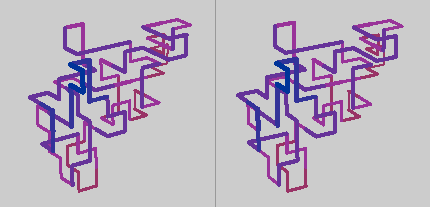
Note: If you cannot perceive the stereo illusion in this illustration, try taking the knot for a spin.
In recent years, faster machinery and superior algorithms have extended the computational studies to larger values of n. Prominent workers in this endeavor have included Whittington and Sumners as well as Neal Madras and E. J. Janse van Rensburg of York University, E. Orlandini and M. C. Tesi of the University of Oxford, and Christine E. Soteros of the University of Saskatchewan. Their numerical experiments have explored the topology of lattice polygons with up to 1,600 sides. Knots remain rare. Even at n = 1,600 hardly more than 1 percent of the random polygons are knotted. Among the knots that do appear, most are simple trefoils, with a handful of figure-eight knots. It seems the fabled asymptotic realm where almost all paths are topologically tangled is still some distance off.
Running a computer experiment in lattice knot theory is a two- stage process. First you generate a bunch of self-avoiding polygons of size n, ideally chosen uniformly from the universe of all n-step self-avoiding polygons. Then you check each polygon to see if it's a knot or not, and perhaps carry out a more precise evaluation of knot type. Both steps have their travails.
Generating an ordinary random walk--one that doesn't worry about crossing its own path--is easy. All you need do is produce a stream of random numbers to select the direction of each step, and keep track of the walker's current position as the path blunders through the lattice. Imposing the condition of self-avoidance seems like a fairly innocent change, but in the end it requires a complete rethinking of the process. For one thing, a program for a self-avoiding walk must have a sense of history; it must keep track of all the sites visited, so that it knows which ones to avoid.
The obvious algorithm for self-avoiding walks is the blind-worm method: The worm chews its way through the interior of an apple, twisting and turning randomly, but it must be careful to back up if it suddenly tastes worm instead of fruit. At each step the procedure is to choose a direction at random, then check to see if the chosen node is already occupied; if it is, back off and try another direction. This algorithm presents two problems. In the first place, it generates a skewed sample of walks, with statistics different from those of a uniform distribution. To correct the imbalance, the procedure has to be altered in a subtle but important way: Instead of merely trying another direction when a conflict arises, the algorithm must throw away the entire walk generated up to that point, and start over. The second problem is even more serious. The advancing end of the walk can stumble into a cul de sac surrounded on all sides by occupied sites, from which it cannot escape. Again there is no choice but to discard the path and start fresh.
Because of these impediments, generating self-avoiding walks is laborious and inefficient. A blind-worm program wastes most of its time on paths that will ultimately fail. And for polygons the situation is even worse. The set of self-avoiding walks that happen to return to their starting point after n steps is a very small subset of all n-step self-avoiding walks.
Accordingly, most work on the geometry and topology of large lattice polygons has been done by other means. Instead of trying to generate many independent random walks, the alternative methods take a single valid walk as a starting point and repeatedly transform it into another valid walk. Depending on what kinds of transformations are applied, the sequence of walks can yield a statistically fair sample of walk configurations, and it wastes no time on rejected paths.
For knot theory the most important method of this kind is called the pivot algorithm. A version for open-ended walks was invented in 1969 by Moti Lal of the Unilever Research Laboratory, and rediscovered by several others in later years. In 1990 the algorithm was adapted to lattice polygons by Madras and A. Orlitsky and L. A. Shepp of AT&T Bell Laboratories. For polygons the algorithm works like this: Pick two vertices at random, thereby dividing the polygon into two segments; then pick one of the segments. Now apply one of several possible transformations to the chosen segment. (The nature of the transformations will be explained shortly.) Finally check to see if the resulting path is still self-avoiding. If it is, accept the move and repeat the entire procedure; otherwise restore the original state and try again by choosing two more random pivot points.
The transformations applied in the pivot algorithm can include rotating the selected segment through some multiple of 90 degrees, or reflecting it in a mirror plane, or inverting it end-for-end. But not all these transformations are possible in all circumstances. For example, rotations work only when the two chosen vertices happen to lie on the same x, y or z axis in the lattice.
The pivot algorithm preserves the length of a polygon but changes its geometry. Of particular importance, the transformations can change the knot type, altering the way strands cross and thread through one another. In 1988 Madras and Alan D. Sokal of New York University proved that the algorithm is ergodic. What this means is that if the algorithm were kept running long enough, it would visit all possible configurations of an n-step polygon. It thus promises a fair sampling of walks. It is also an efficient method. The number of operations needed to generate each new configuration is proportional to n log n.
The fundamental problem of knot theory, both on and off the lattice, is determining whether two knots are equivalent--whether one can be deformed so that it looks just like the other. After a century of study the problem remains unsolved: There is no foolproof algorithm for classifying knots. [Correction] This is rather awkward for computer programs that need to recognize knot types.
In practice, the programs make do with classification methods that are less than totally reliable. The most common method is to calculate a knot's Alexander polynomial. (The Alexander in question here is not the one who famously cut the Gordian knot; he is the American mathematician J. W. Alexander, who devised the polynomial in the 1920s.) The Alexander polynomial is calculated from a two-dimensional projection of a three-dimensional knot. Think of the projection as the shadow cast by the knot, but annotated wherever two strands cross to show which strand passes over and which under. The annotated projection incorporates all the essential information about the knot, but a given knot can have many different projections. The Alexander polynomial provides an invariant: All the projections yield the same polynomial. For example, any projection of the trefoil has the Alexander polynomial t - 1 + t-1, and the polynomial of the unknot is simply 1.
It's helpful that every projection of a knot has the same polynomial, but what the knot theorist would really like to hear is that every polynomial corresponds to just one knot. Then calculating the polynomial would unambiguously identify the knot. Unfortunately, there are pairs of distinct knots that share the same Alexander polynomial; there are even knots with the same polynomial as the unknot. Thus relying on the Alexander polynomial to identify knots risks occasional error.
Even if an exact algorithm for classifying all knots is out of reach, perhaps one might at least be able to distinguish knots from unknots? The Alexander polynomial cannot do this with total reliability, but a polynomial introduced in 1985 by Vaughan F. R. Jones of the University of California at Berkeley may discriminate more finely. So far, no one has found a nontrivial knot whose Jones polynomial is the same as that of the unknot. But a proof is lacking, and counterexamples are expected.
There is an algorithm guaranteed to determine whether a given knot is the unknot, but it has never been implemented in a computer program. The algorithm was published in 1961 by Wolfgang Haken, now of the University of Illinois at Urbana-Champaign (and the co-solver of another famous problem in topology, the four-color-map theorem). The paper describing the algorithm is 130 pages of German, which I do not read, and so my knowledge of it has been limited to scraps gleaned from secondary literature and lore.
Recently, Haken's algorithm has been analyzed--and, incidentally, explicated--by Joel Hass of the University of California at Davis, Jeffrey C. Lagarias of AT&T Laboratories and Pippenger. The essence of the algorithm is to examine the two-dimensional surface whose boundary is the closed path being tested for knottedness; if this surface is topologically equivalent to a disk, then the path is the unknot. Haken gave a procedure for determining whether or not the surface is a disk. Hass, Lagarias and Pippenger find that the running time of a program based on this procedure would be proportional to 2 raised to the power cr2, where c is a constant and r is the number of crossings in the knot diagram. They also derived a modified algorithm with the running time 2cr. Even with this improvement, however, the algorithm is not one you would want in the inner loop of a program.
My preference for doing topology on a lattice doubtless reflects my personal tastes and prejudices, as well as the limits of my imagination. But perhaps the limits of computers are also a factor here (if not their tastes and prejudices).
Consider how a computer program calculates the Alexander polynomial of a knot. First it creates a two-dimensional projection, then it traces through the projection, stopping at each crossing point to write a term of the polynomial. When I learned how the projection is made, I was appalled. The first step is to rotate the lattice in R3 through angles with irrational cosines. There goes the tidy world of integer coordinates!
There's a good reason for the rotation. A knot viewed along one of the lattice axes is incomprehensible, because points stack up on top of each other. (Note that in the illustrations for this article, knots are seen from oblique points of view.) The irrational rotation ensures that all crossings in the projection are "regular," with no more than two edges meeting at a point. But regularity has a price: All the amenities of working with integer coordinates are lost. On a lattice, every intersection of lines must lie at one of the nodes, and so an algorithm for finding crossing points has only to compare integers for numerical equality, an operation that can generally be done with total accuracy in a single machine instruction. Finding intersections in R3 is more difficult, as it requires solving simultaneous equations. Furthermore, the solution found may be only an approximation to the true point of intersection, especially if that point has irrational coordinates. Janse van Rensburg and Whittington have reported that one of their programs spends most of its time looking for crossings in knot projections.
A final irony is that the cosines in the rotation matrix are not really irrational. For computational convenience, the program employs a rational approximation. So we never really leave the lattice after all; we just see the world through a much finer mesh.
(Note: The bibliography given here includes additional references not present in the printed version of this article.)
Adams, Colin C. 1994. The Knot Book: An Elementary Introduction to the Mathematical Theory of Knots. New York: W. H. Freeman.
Alexander, J. W. 1928. Topological invariants of knots and links. Transactions of the American Mathematical Society 30:275-306.
Dasbach, Oliver T., and Stefan Hougardy. 1997. Does the Jones polynomial detect unknottedness? Experimental Mathematics 6:51-56.
Delbrück, M. 1962. Knotting Problems in Biology. Proceedings of Symposia in Applied Mathematics, Vol. 14, pp. 55-63. Providence: American Mathematical Society.
Diao, Yuanan. 1993. Minimal knotted polygons on the cubic lattice. Journal of Knot Theory and its Ramifications 2:413-425.
Diao, Yuanan. 1994. The number of smallest knots on the cubic lattice. Journal of Statistical Physics 74:1247-1254.
Frisch, H. L., and E. Wasserman. 1961. Chemical topology. Journal of the American Chemical Society 83:3789-3795.
Haken, W. 1961. Theorie der Normalflachen. Acta Mathematica 105:245-375.
Hammersley, J. M. 1961. The number of polygons on a lattice. Proceedings of the Cambridge Philosophical Society 57:516-523.
Hass, Joel, Jeffrey C. Lagarias and Nicholas Pippenger. 1997. The computational complexity of knot and link problems. Presented at the 38th Conference on Foundations of Computer Science, October 20-22, 1997, Miami Beach, Florida.
Janse Van Rensburg, E. J., E. Orlandini, D. W. Sumners, M. C. Tesi and S. G. Whittington. 1996. Entanglement complexity of lattice ribbons. Journal of Statistical Physics 85:103-130.
Janse Van Rensburg, E. J., M. C. Tesi, E. Orlandini, D. W. Sumners and S. G. Whittington. 1997. The writhe of knots in the cubic lattice. Journal of Knot Theory and its Ramifications 6:31-44.
Janse van Rensburg, E. J., and S. D. Promislow. 1995. Minimal knots in the cubic lattice. Journal of Knot Theory and its Ramifications 4:115-130.
Janse van Rensburg, E. J., and S. G. Whittington. 1990. The knot probability in lattice polygons. Journal of Physics A: Mathematical and General Physics 23:3573-3590.
Janse van Rensburg, E. J., S. G. Whittington and N. Madras. 1990. The pivot algorithm and polygons: results on the FCC lattice. Journal of Physics A: Mathematical and General Physics 23:1589-1612.
Jones, Vaughan F. R. 1985. A polynomial invariant for knots via von Neumann algebras. Bulletin of the American Mathematical Society 12:103-111.
Jones, Vaughan F. R. 1990. Knot theory and statistical mechanics. Scientific American 263(5):98-103, November.
Kesten, Harry. 1963. On the number of self-avoiding walks. Journal of Mathematical Physics 4:960-969.
Lacher, R. C., and D. W. Sumners. 1991. Data structures and algorithms for computation of topological invariants of entanglements: link, twist and writhe. In Roe, R. J. (editor), 1991, ComputerSimulation of Polymers. Englewood Cliffs, N.J.: Prentice Hall.
Lal, Moti. 1969. "Monte Carlo" computer simulation of chain molecules, I. Molecular Physics 17:57-64.
Lickorish, W. B. R., and K. C. Millett. 1988. The new polynomial invariants of knots and links. Mathematics Magazine 61(1):3-23, February.
Madras, N., A. Orlitsky and L. A. Shepp. 1990. Monte Carlo generation of self-avoiding walks with fixed endpoints and fixed length. Journal of Statistical Physics 58:159-183.
Madras, Neal, and Gordon Slade. 1993. The Self-Avoiding Walk. Boston: Birkhäuser.
Madras, Neal, and Alan D. Sokal. 1988. The pivot algorithm: A highly efficient Monte Carlo method for the self-avoiding walk. Journal of Statistical Physics 50:109-186.
Millett, K. C., and D. W. Sumners (editors). 1994. Random Knotting and Linking. Singapore: World Scientific.
Orlandini, E., M. C. Tesi, E. J. Janse van Rensburg and S. G. Whittington. 1996. The entropic exponents of lattice polygons with specified knot type. Journal of Physics A: Mathematical and General Physics 29:L299-L303.
Pippenger, Nicholas. 1989. Knots in random walks. Discrete Applied Mathematics 25:273-278.
Slade, Gordon. 1996. Random walks. American Scientist 84:146-153.
Soteros, C. E. 1997. Knots in graphs in subsets of Z3. To appear in IMA Volumes in Mathematics and its Applications. Preprint available at http://math.usask.ca/~soteros/
Soteros, C. E., and M. M. Paulhus. 1996. A Monte Carlo algorithm for studying the collapse transition in lattice animals. To appear in IMA Volumes in Mathematics and its Applications. Preprint available at http://math.usask.ca/~soteros/
Soteros, C. E., D. W. Sumners and S. G. Whittington. 1992. Entanglement complexity of graphs in Z3. Mathematical Proceedings of the Cambridge Philosophical Society 111:75-91.
Sumners, D. W., and S. G. Whittington. 1988. Knots in self-avoiding walks. Journal of Physics A: Mathematical and General Physics 21:1689-1694.
Sykes, M. F., D. S. McKenzie, M. G. Watts and J. L. Martin. 1972. The number of selfavoiding rings on a lattice. Journal of Physics A: General Physics 5:661-666.
Tesi, M. C., E. J. Janse van Rensburg, E. Orlandini and S. G. Whittington. Knot probability for lattice polygons in confined geometries. 1994. Journal of Physics A: Mathematical and General Physics 27:347-360.
Vologodskii, A. V., A. V. Lukashin, M. D. Frank-Kamenetskii and V. V. Anshelevich. 1974. The knot problem in statistical mechanics of polymer chains. Soviet Physics--Journal of Experimental and Theoretical Physics 39:1059-1063.
Wasserman, E. 1962. Chemical topology. Scientific American 207 (November):94-102.
Whittington, Stuart G. 1992. Topology of polymers. Proceedings of
Symposia in Applied Mathematics 45:73-95.
© 1997 Brian Hayes